
A continuous cloud chamber shows tracks of charged particles. Advance notice is needed to obtain the dry ice necessary to operate the chamber. Thoron gas (thorium emination, Rn 220, half-life = 1 min.) can be blown into the chamber to produce alpha particle tracks. Since the daughter nucleus Po 216 with a half-life of 0.15 sec. is also an alpha-emitter, two pronged tracks will be seen in the chamber. A needle with Pb 210 also produces a-tracks. Two to five students look at this demonstration at once so it is best to arrange a little time at the beginning or end of class for them to come down and look.
Cloud Chamber
Methanol evaporates from the trough, and the vapor falls toward the cold dry ice (-100 F = -73 C). In the process the vapor is super cooled; that is, cooled below its normal condensation point. When a high speed charged particle from a radioactive source or from a cosmic ray passes through the super cooled vapor, it ionizes the air and methanol atoms along the way; i.e., it strips electrons from these atoms. These ions and electrons serve as condensation centers for the methanol vapor, which condenses out in tiny droplets along the track of the charged particle outlining its path.

The charged particles from the radioactive source are typically helium nuclei (alpha particles). This source is "license free", meaning it is too weak to be considered dangerous by governmental regulatory agencies. Charged particles from cosmic rays are typically protons and muons.
Using the color projector (Projected Colors [1]), you can simulate the quark structure of baryons and mesons.
Heavy water, D2O, molecular weight 20, is about 10% heavier than ordinary water, H2O, molecular weight 18. Identically filled bottles of heavy water and tap water can be compared by hand or on a double pan balance. Of course, deuterium and heavy water are not radioactive.
The Physics Demontrations Group has a collection of videos on nuclear physics including:
The Physics Demontratons Group has a collection of transparencies on nuclear physics copied from Scientific American and other books including:
Small "license free" sources of activity < 0.1 microcurie can be taken into the class to activate a small hand held counter. Cloud chamber alpha sources of lead 210, beta source of strontium 90, thoriated tungsten welding rod, uranium glass (alpha beta gamma), Americium (alpha gamma) from a smoke detector and a hot fiesta ware cup and saucer with uranium glaze are available.
Americium-241, with a half-life of 432 years, is used in most domestic smoke detectors. Am-241 decays by emitting alpha particles and 60 keV gamma radiation to become neptunium-237.
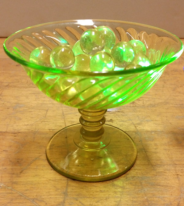
Uranium glass was used to make a yellow tinted dinnerware from Victorian times. Sometimes called Vasoline glass, or depression glass, our bowl measures about 5 µSv/hr. You can tell uranium glass because it fluoresces green under blue or UV light.
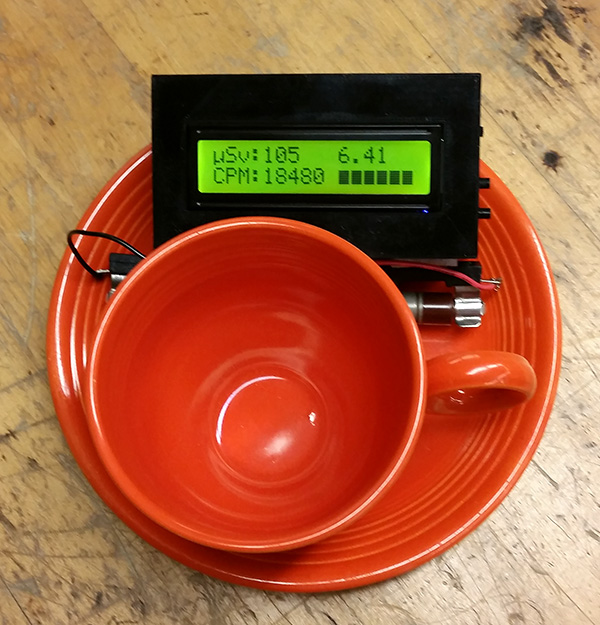
Fiesta ware was the largest selling dish line in American history – 200 million dishes were shipped since 1936. The red/orange color glaze contains uranium. The government seized the company's uranium supply in 1943 out of fear it could be used to make a bomb. A single plate contains about 4.5 grams of uranium, mostly U-238. Production resumed in 1959 with depleted uranium (depleted of U-235) and continued until 1972 when it was discontinued out of concerns about uranium and lead leaching out of the glaze. Fiesta ware is the hottest source we have and measures over 100 µSv/hour at the plate surface, but this is not considered dangerous for display purposes. U-238 has a half-life of 4.5 billion years.
Radiation safety standards limit public exposure to 1 mSv/year and occupational exposure to 50 mSv/year. Natural background radiation is about 3 mSv/year.
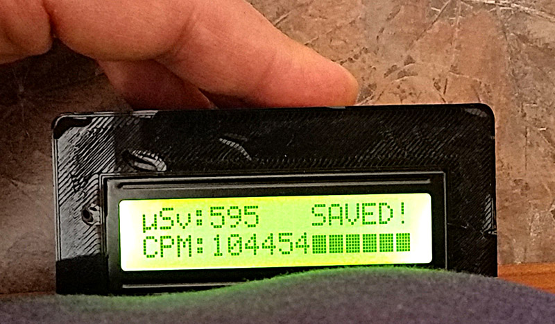
Contrast that with a typical medical dose as shown below. This reading was taken about two hours after injection with Technetium-99m, a radioisotope used for heart imaging with a 6 hour half life.
A handheld Gieger-Mueller tube is available.
Lewis Carroll Epstein in his book Relativity Visualized has developed several marvelous illustrations curved spacetime. Art has a copy of the book and model transparencies that you can curve and flatten out on the overhead projector to show:
A description of 4-Dimensional space
See Local Inertial Frame (Gravitational Acceleration) [2]. This demonstration is equivalent to the Monkey and Hunter [3] example. A large aluminum frame is cranked up and suspended by a magnet. Two guns on one side of the frame are aimed in straight lines through holes in an intermediate Plexiglas sheet at target pockets on the other side of the frame. If the guns are fired while the frame is suspended, the projectiles travel in parabolas and bounce back from the plastic sheet. But now the guns are reloaded and frame is released to fall. Another switch fires the guns as the cage goes into free fall. When the falling frame is stopped by a "linear decelerator" (a shock absorber) at the bottom, it will be found that the projectiles reached the pockets. In the falling frame, they traveled in straight lines, obeying Newton's First Law.
Our device was designed by Dr. R.E. Berg of the University of Maryland (A.J.P. 48, 310 (1980)), and built by the UCLA physics machine shop.
Attention can be called to the well-known Monkey and Hunter [4] demonstration as an illustration of the Principle of Equivalence (POE). The impressive point is that no complicated ballistic calculation is needed. Consider a reference frame falling with the bullet and the monkey. (Imagine a frame released the instant the bullet leaves the muzzle and the monkey starts falling.) In this frame the bullet is initially directed at the monkey and travels uniformly in a straight line toward it. By the POE this falling frame is truly inertial and the fact that the bullet hits the monkey is an immediate consequence of Newton's First Law. (A. Huffman, A.J.P. 48, 314 (1980))
Two very simple demonstrations of weightlessness when falling are described in Weightlessness (Gravitational Acceleration) [5].
This is a 16 minute NASA video of physics experiments in the orbiting laboratory of Sky lab. Weightlessness is well shown, and the rest is a physics 10 level discussion of gravity, satellite motion, and illustrations of Newton's laws in weightlessness.
This demonstration uses the microwave apparatus of experiment 2 in the 8D lab. The microwaves produced by a Gunn diode are picked up by a receiver and indicated on a meter visible to the class. When one of the 45 degree prisms is inserted into the beam, the meter reading drops to near zero - the microwaves have been totally internally reflected at right angles. You can demonstrate that this is the case by moving the receiver around to the right-angle position to pick them up. Now the receiver is returned to the original position, and a second prism is brought close to the first as shown above. When the gap is about one centimeter or less, the signal begins to increase - the microwaves have tunneled across the gap into the second prism. When the gap distance is reduced to zero, the signal reaches its full value. As the gap distance is increased, the signal drops off exponentially.
Remember, even electromagnetic microwaves are photons! This is a demonstration of particles penetrating a barrier.
The black body radiation curve can be demonstrated by using a radiation sensor hooked to a digital millivoltmeter. The carbon disulfide prism [6] is used to spread out the light of a slide projector lamp onto a screen . As you scan across the spectrum with the radiation sensor, the millivoltmeter shows the peak of the 3000 K tungsten filament in the infrared with the tails of the curve in the visible spectrum and further infrared.
The same demonstration can be done more qualitatively. Turn down the room lights and show the spectrum of "white" light on the wall. As you reduce the voltage to the lamp with the variac, the blue color dies away, and then the green, leaving only dull red of low intensity. (Of course, the 3000 K tungsten filament already peaks in the infrared so the initial "white" light is already quite red. Infrared itself can be demonstrated; see Infrared, Radiometer, and Maxwell's Spectrum [7])
|
The applet below shows the blackbody curve and colors corresponding to the given temperature. |
|||
|
When introducing the Bohr atom it is a good idea to review standing waves for the students, for example with Rudnick's String [9]. You can show how the string resonates for various harmonics as the driving frequency is changed.
Another demonstration puts standing waves on a circular wire loop - standing waves around a circle. A mechanical wave driver controlled by a function generator shakes the loop at the bottom and it resonates with an odd number of antinodes on the circle at the frequencies:
| Number of antinodes | Frequency (Hz) |
| 3 | 18 |
| 5 | 65 |
| 7 | 140 |
| 9 | 237 |
The set-up below is an excellent demonstration of the wave nature of particles. An electron beam is passed through a carbon foil and the resulting diffraction rings displayed on the fluorescent screen of the tube. (Since the graphite crystals are randomly oriented, the diffraction pattern is rings.) From the accelerating voltage, DeBroglie's wavelength, and the diffraction ring diameter, you can calculate the atomic spacing of carbon.
The students don't know what they are seeing. You take that into the class room and the students see green rings, but a physicist sees something astonishing, the wave nature of matter.
-Prof. George Igo
Students can see the spectral lines of hydrogen by looking at a arc tube on the lecture table through replica gratings. Several students can come down at once and look. You can also project the spectrum of mercury on a screen for the whole class to see (See Projected Mercury and Continuous Spectra [10]).
A simple demonstration of energy levels can be done with 4 LEDs, a handcranked generator, and a supercapacitor. As the capacitor is charged by the generator, first the red LED lights, then the green, then the blue. As the capacitor discharges, first the blue led goes dark, then the green, then the red. There is also a fourth IR LED which can't be seen by the eye, but can be seen on a cell phone camera or video camera when the room lights are out. It turns on first and turns off last. Each color has an energy (voltage) threshold which is related to the photon energy. The IR turns on at 1.2 V, red at 1.5 V, green at 2.0 V, and blue at 3.5 V.
The Frank-Hertz Experiment [11] shows atomic energy levels, but it is a very complicated demonstration.
Finally, a very simple demonstration of energy levels is fluorescent and phosphorescent materials with an ultraviolet light. The energetic UV light kicks the electrons up into high levels, and as they jump part way down immediately (fluorescent) or with some seconds of delay (phosphorescent with partially forbidden transitions), the electrons emit visible light of various colors. A green phosphor requires a blue or ultraviolet light to be activated. A red or green LED or laser won't make it glow, but a blue LED will.

This classic 1914 experiment showed the existence of energy levels and their association with spectral lines. It involves an elaborate setup which requires over an hour of warm-up time and calibration. It is best suited for a lab experiment, or you could arrange to have it set up in a lab, and then bring the students in to watch it. Give plenty of extra notice.
Electrons are accelerated in a nearly evacuated tube with a little mercury vapor in it from the cathode to anode by the voltage V. Those reaching the collector are retarded by 0.5 V. Thus, as V is increased from zero, there is no collector current at A until V > 0.5 V. Then the collector current rises until V reaches the excitation potential of a level in the gas atoms. The inelastic collisions reduce the electrons' energy to zero, and the current drops. As V is increased further, the current again increases until the electrons reach the energy of another level, or double that of the first level. The results can be seen on the current meter as the voltage is increased, or displayed on an oscilloscope screen using a sweep voltage.
A very simple demonstration of the photoelectric effect is performed with a zinc plate as the electrode of an electroscope. An ultraviolet lamp covered with glass is arranged to shine on the plate. The plate is charged negative with an electrophorus, and the electroscope needle diverges indicating the charge. The blue light of the lamp will not knock out electrons from zinc, but if the glass (opaque to UV) is removed from the lamp, the needle quickly falls as electrons are kicked away from the plate. The zinc plate must be cleaned with steel wool within an hour or so of the demonstration to remove the oxide.
A variation of this experiment has a spiral electrode with a positive voltage in front of the zinc plate with a sensitive current meter to measure the small current of the photoelectrons through the air.
The photoelectric effect is also done as experiment 4 in the 8E lab. The stopping voltage is measured as a function of wavelength (color) of the exciting light, and Planck's constant determined from the slope of the line.
The Ripple Tank [12] is useful to remind the students of wave interference. You might also wish to use the Acoustic Interference [13] demonstration with the ultrasonic transducers. With this setup, you can show that covering one of the two sources will increase the signal to the detector in the case of destructive interference, a key property of waves.
Light has wave properties: show interference with laser shining through slits (See Interference and Diffraction [14]).
Light has particle properties: show the Photoelectric Effect [15].
Electrons have wave properties: show Electron Diffraction [16].
The ratio of e/m for an electron can be measured with an apparatus consisting of a spherical evacuated electron tube mounted inside of a Helmholtz coil setup. The electrons are projected to circle in the magnetic field, and you measure the radius of the circle, the current to the Helmholtz coils, and the accelerating voltage to determine e/m. (See also E/M and Helical Electrons [17].) This is experiment 2 in the 8E lab.
An operating interferometer can be demonstrated in the classroom. It is too small for the actual Michelson-Morley experiment, but you can display to the class interference fringes that change as one of the mirrors is moved.
Two good films for relativity are "Frames of Reference" and "Time Dilation". The first is an excellent older film lasting for 30 minutes showing experiments in Galilean relativity filmed from different points of view, the laboratory frame, uniformly moving, accelerated, and rotating frames. Paul Hewitt's Time Dilation film lasts about 15 minutes and resolves the twin paradox by the Darwin method, counting light signals emitted at regular intervals by the other twin. A description of the twin experiment and calculation of the times is repeated in Hewitt' s book, Conceptual Physics.
Also available are the highly instructive Mechanical Universe series on relativity chapters 42 and 43.
"The influence of the crucial Michelson-Morley experiment on my own efforts has been rather indirect. I learned of it through H.A. Lorentz's decisive investigations of the electrodynamics of moving bodies (1895) with which I was acquainted before developing the special theory of relativity . . . What led me more or less directly to the special theory of relativity was the conviction that the electromotive force acting on a body moving in a magnetic field was nothing else than an electric field.
-Albert Einstein
Although most physicists are aware that relativity is involved in the Faraday magnet and coil induction experiment [18], few exploit the full significance of it as a relativity demonstration. But this experiment demonstrates a truly relativistic effect at very low velocities. It shows, among other things, that physical results depend only on the relative motion (Einstein's first postulate of relativity, the physics is independent of the uniform motion of an inertial frame), and that electric and magnetic fields manifest themselves differently to different moving observers. In addition the experiment has the advantage of motivating relativity in the same way as Einstein was motivated, as in the quote above. This demonstration is useful as a general introduction to relativity in the non-calculus courses and as a motivation for the Lorentz transformation in a higher level special relativity course.
A good place to introduce the demonstration for the first time is just before the coverage of Faraday Induction. (Later when relativity is covered, the demonstration can be repeated and new features emphasized. Referring to the figure first hold the magnet stationary with respect to the classroom, and move the coil toward the magnet. In this situation, case A, the force that moves the electrons around the coil to produce the galvanometer readings the Lorentz force F = qv/c X B. where v is the velocity of the coil toward the magnet.
Before demonstrating the moving magnet case B, discuss with the students what they should expect to see. There is a magnetic field, but this does not affect the electrons in the coil, since their velocity is initially zero, and even after they begin to circulate around the coil, the magnetic v X B force is perpendicular to the wire and so does not cause the current. In fact, nothing the students have studied so far in E & M would lead them to expect a galvanometer reading in case B. When this proposition is put to the class, some students will object that " it shouldn't matter whether the coil or magnet is moved". If the class is pressed on this point, one can usually draw out the comment that "only the relative motion should matter". After a short discussion of Einstein's relativity principle, one can go on to perform case B. moving the magnet toward the coil. But, of course, although Einstein's postulate tells us that there must be a new force on the electrons, this new force must have a specific physical origin or description, and it is then appropriate to introduce Faraday induction or Grad X E = 1/c dB/dt. (In a non-calculus course this can be simply worded as a changing magnetic field produces a circular electric field.)
Further points that can be emphasized when the experiment is demonstrated later for relativity are:
The principles of this demonstration as presented in a non-calculus course are summarized on the next page which is available as a transparency from Art.
This demonstration was inspired by section 16.7 of Basic Physics by Kenneth W. Ford (Blaisdell Publishing Co., Waltham, Mass., 1968) The Einstein quote quote at the beginning was from the 1952 meeting honoring the centenary of Michelson's birth as quoted in Introduction to Special Relativity by Robert Resnick (John Wiley and Sons, New York, 1968).
(Art Huffman, AJP 48, 780 (1980))
We see Lucy and Ringo both moving, approaching each other.
Lucy says:
The loop is stationary and the magnet is moving toward it. There is a magnetic field, but it can't produce any force on my electrons since they are stationary within the loop. Instead, the magnetic field is changing, growing stronger as the magnet gets closer, and this changing magnetic field produces an electric field which causes forces on the electrons, and drives them around the loop and produces the current in the galvanometer.
Ringo says:
The magnet is stationary and the loop is moving toward it. The electrons in the loop, since they are moving with the loop, feel a magnetic force, F = - e/c v X B, which drives them around the loop and produces the current in the galvanometer. There is no electric field.
The Conclusion:
Electric and magnetic fields are not invariant entities themselves, but are aspects of a single entity, the electromagnetic field, which manifests itself differently to different moving observers.
Links:
[1] https://demoweb.physics.ucla.edu/node/370
[2] https://demoweb.physics.ucla.edu/node/411
[3] https://demoweb.physics.ucla.edu/node/456
[4] https://demoweb.physics.ucla.edu/node/387
[5] https://demoweb.physics.ucla.edu/node/414
[6] https://demoweb.physics.ucla.edu/node/208
[7] https://demoweb.physics.ucla.edu/node/207
[8] http://webphysics.davidson.edu/Applets/Applets.html
[9] https://demoweb.physics.ucla.edu/node/278
[10] https://demoweb.physics.ucla.edu/node/84
[11] https://demoweb.physics.ucla.edu/node/86
[12] https://demoweb.physics.ucla.edu/node/339
[13] https://demoweb.physics.ucla.edu/node/52
[14] https://demoweb.physics.ucla.edu/node/90
[15] https://demoweb.physics.ucla.edu/node/209
[16] https://demoweb.physics.ucla.edu/node/461
[17] https://demoweb.physics.ucla.edu/node/212
[18] https://demoweb.physics.ucla.edu/node/197