Two solenoid coils connected by wires are arranged so that magnets on springs oscillate in them. When one magnet is set oscillating, the induced current causes the other to oscillate also. Note that the oscillations are coupled through the velocity term rather than the amplitude term as in coupled pendula.

Also Current Coupled Coils (Electrodynamics) [1]

A Pasco apparatus gives digital readouts of the natural period of the oscillator, the driving frequency, and the amplitude of oscillation. A flashing LED shows the phase angle between driving force and the oscillator. This is the type of instrument that is even more interesting to the professor than the students. The driving frequency and amplitude, spring constant, mass, and damping can all be varied. You can quantitatively measure amplitude versus time (undriven), amplitude versus driving frequency, phase angle versus driving frequency, transient response, etc.

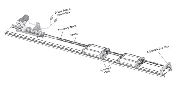
We also have a horizontal version with variable magnetic damping, using the Pasco track and a cart connected by a spring to a sinusoidal drive. This version has no electronic readout.

With this nice piece of apparatus you can vary the driving frequency and amplitude, and the damping (electromagnetic). Essentially the same concepts as above can be illustrated, minus the electronic readouts.

This demonstration is similar to Laser Sine Wave from Tuning Fork [2], but the tuning fork is now driven by a magnet coil connected to an audio oscillator. Normally the beam is not scanned with the rotating mirror, but one merely observes the amplitude of oscillation on the wall. One can demonstrate resonance by observing the large increase in amplitude when the oscillator is tuned to the natural frequency of the fork. If the oscillator is tuned slightly off resonance, beats between the driving frequency and the natural frequency are observed.

This impressive demonstration shows that the simple harmonic motion of a tuning fork is really a sine wave in time. A laser beam is bounced off a mirror on the end of a tuning fork to a rotating mirror which provides the time axis. The tuning fork is driven by an interrupted magnet.

- This information is from Bob Keolian.

The trick is in the suspension. At the "Mystery Spot," a tourist trap in Santa Cruz, they suspend the pendulum with a chain by casually looping the chain around a horizontal beam associated with the roof of a shed. The chain reattaches to itself, forming a "V" at the top. Your's must do something similar, forming a V at the top, with two fixed attachments at the top of the V and a knot or some other junction at the bottom of the V to a single chain or rope that goes down to the pendulum. The trick is in noticing that for motion perpendicular to the plane of the V, the effective length of the pendulum is from the two attachments at top to near the center of mass of the pendulum below, but for motion in the plane of the V, the junction or knot point remains fixed and the effective length of the pendulum starts from there. This gives a shorter length and slightly higher frequency for motion in the plane of the V than for motion perpendicular to the plane of the V.

At reasonably small amplitudes, say less than about 10 degrees of deflection, the motion of the pendulum can be considered to be a linear superposition of in-plane and out-of-plane motion, with two modes of slightly different frequencies. So you can get different Lissajous figures depending on how you start off the pendulum. If you start off with a circular motion, you are exciting both modes with the same amplitude but with an initial 90 degree phase shift between them. As the modes progress in time, the instantaneous phase between them (w_1t - w_2t - initial phase) changes with time. Eventually, the two modes are in phase and the pendulum move in a straight line 45 degrees from the plane of the V. Later the phase is such that the circle changes direction. If you let the pendulum go, the pattern repeats itself. But that isn't as much fun as stopping the pendulum after it has reversed direction once and cooking up some BS story about a gravitational or magnetic anomaly in the mantle below Los Angeles that causes the change in direction.

If you start the pendulum off in planer motion either in the plane of the V or out of the plane of the V, then you excite only one of the modes, and the motion stays in its plane. At larger amplitudes the linear superposition of modes picture breaks down, at around 30 degrees of deflection. The two modes couple parametrically by modulating the tension in the rope at twice the oscillation frequency, but that is another story.

Parametric oscillation occurs when one of the parameters of the system is varied. A child can "pump" a swing by standing and raising and lowering her center of mass periodically, changing the length of the pendulum. The child pumps at twice the pendulum frequency, generating a sub harmonic.

A very simple demonstration of parametric oscillation is the coupling of the pendulum mode to a mass on a spring. When the spring frequency is approximately twice the swinging frequency (pendulum mode), the spring mode parametrically drives the pendulum mode, but the pendulum motion causes the tension in the spring to vary at twice the pendulum frequency, and therefore resonantly drives the spring mode. The transfer of energy between these two modes is impressive.

This exhibits wave like behavior, but the wave is an illusion. The pendulums are independent.

1. The Driven Mass on a Spring [3] can be easily set to resonance. Measure the natural period with the LED readout and then drive at the inverse, the natural frequency, also measured by the LED readout. Or adjust the phase between the driver and oscillator to 90 degrees lag as shown by the phase readout.

2. Resonance can also be found for the Driven Torsion Pendulum [4]. This is a little more difficult since there are no electronic readouts and the Q of the torsion wheel is quite large.

3. The Driven Tuning Fork [5] demonstrates resonance at high Q. as the frequency synthesizer is adjusted in steps of 0.1 Hz near its resonant frequency.

4. In Beats and Sympathetic Vibration [6], see show how one vibrating tuning fork can acoustically induce vibrations in another nearby, if it is tuned to the same frequency.

5. A dramatic demonstration of resonance in Breaking Glass with Sound [7].

Along with this we have the Tacoma Narrows Bridge collapse on video.

 

6. The Pasco track can be connected to a sinusoidal drive to demonstrate a driven simple hormonic oscillator. When the motor drive matches the resonance of the system, energy gets pumped in and the amplitude of the oscillations grow dramatically. This system can also be used to show a critically damped and under damped system by bringing an aluminum sheet close to two magnets attached to the cart.

 

 

7. A new demonstration is "resonance strips". Several metal strips of increasing length are bolted together in a star shape. When the device is vibrated with a mechanical driver controlled by a signal generator, the different strips come to resonance in the range 10 50 Hz by vibrating strongly at different frequencies according to their lengths. The class can see the frequency of the driver on a large display frequency counter.

8. The mechanical driver will also vibrate a ten inch wire loop, and will induce standing waves with 3, 5, 7, etc. antinodes around the circle at specific increasing frequencies. Rudnick's String [8] shows the same effect on a linear string.

 

The following demonstrations are available to show simple harmonic motion.

	a. Analogy of Simple Harmonic Motion to Circular Motion: A device which you crank around fits on a projector. One dot moves around the circle while another dot projected on a diameter stays underneath the first dot and executes simple harmonic motion.
b. Mass on a Spring: Springs of two different spring constants are supplied along with several weights. A ruler device can be used with different weights on the springs to measure their k's. With a 200 g mass on the stiffer spring, the spring mode and pendulum mode are parametrically coupled.

f. Torsion pendulum: the weights can be moved as shown to change the rotational inertia, and therefore the period.

g. Coupled pendula: Three varieties are available.

1. Two pendula coupled by a spring (shown to the right) will show normal modes, and transfer of energy between the single pendula swinging modes.

   

2. A mass on a spring has the vibrating spring mode resonantly coupled to the pendulum mode. This is an example of parametric oscillation [11]. The spring frequency is approximately twice the swinging frequency (pendulum mode). The spring mode parametrically drives the pendulum mode, but the pendulum motion causes the tension in the spring to vary at twice the pendulum frequency, and therefore resonantly drives the spring mode. The transfer of energy between these two modes is impressive.

   

3. A Wilberforce pendulum has the vibrating spring mode coupled to a torsion pendulum mode.

   

h. Coupled gliders on an air track: Two gliders with three springs, two running to the fixed ends and the third between show normal modes and exchange of energy.

i. Some Unusual Pendula: Suggested by Bruce Denardo

1. An inverted pendulum; that is, a vertical stick, free at the top, whose support is vertically vibrated, can be stabilized about a vertical position.

   

2. Precession of a spherical pendulum a spherical pendulum is a conical pendulum set swinging in an ellipse. For small amplitudes the periods along the major and minor axes are almost equal and the ellipse remains stationary in space. But for large amplitudes the ellipse precesses forward because the period for planar pendulum motion on the major axis is somewhat larger than that along the minor axis. (The period of a planar pendulum increases somewhat with amplitude as the small angle small oscillation approximation fails.)

   

3. The Mystery Spot Pendulum is named after a supposed site of gravitational anomaly in Northern California. A conical pendulum first swings in a circle one way, then gradually reverses to circle the other way. (Demystification courtesy of Bob Keolian.) [12]

   

Simple pendulum, conical pendulum, collisions, Lissajous figures, and others can all be illustrated with this interesting demonstration. See Two Balls Hanging (Momentum and Collisions) [13]

[13]