| A four meter long track is available for Galileo's "diluted gravity". Galileo argued that as the angle of incline of a track is increased, the motion of a rolling ball approaches free fall, so that the motion of the ball down the track is the same type of accelerated motion as free fall.
This device is very useful when you are discussing uniformly accelerated motion and free fall because motion is slow enough on the track so you can describe it while it is happening. For example, you can simulate a ball thrown in the air by rolling a ball up the track while discussing how its velocity decreases on the upward leg, becomes zero at the top, and increases on the downward leg. |
|
The concept of acceleration can be demonstrated by rolling a ball down the inclined plane and marking its successive positions on drafting tape pasted to the track, timing the positions with metronome beats. The simplest way to do this is to have several positions marked before the class begins and add a few more during the class demonstration, while showing the students that the ball passes all the marks at the right times. Then by measuring the distances you can show that the total distance the ball rolls increases with the square of the time.
Galileo's experiment itself is likely to be obscure to the students, since it depends on knowing that the difference of successive square integers are the odd integers. It can be performed as follows: The tape pasted to the track is marked as before, or perhaps by a student volunteer with good reaction time and coordination. The tape is then cut at the marks and pasted onto the blackboard in the form of a bar graph. The ratios of the heights 1 : 3 : 5 : 7 : 9 ... give the differences of the squares in the formula y = 1/2 at2.
A sonic ranger measures the distance to a moving object by bouncing ultrasonic sound off the object and timing the echoes. The data, taken about every 0.05 sec. is read into a computer which then plots the distance, velocity, and acceleration. The results can appear on overhead projection via the LCD screen, or in some rooms, directly on video projection. Derivatives, integrals and other manipulations of these quantities can be performed. Three typical experiments are described:
|
|
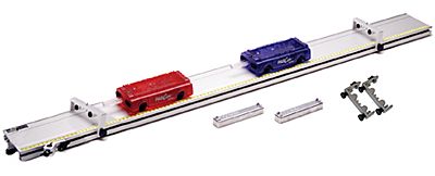
1. A cart is sent up a tilted Pasco track to roll back down. This is a good demonstration to illustrate kinematics concepts since the students can see distance, velocity, and acceleration plotted simultaneously. |
| 2. A plate is supplied which the instructor can move in various ways to again illustrate d, v, and a. Start simple; hold the plate at constant position for a few moments, move at constant velocity to a new position, and hold this new position for a few moments. Have the students predict the graphs of d,v, and a. |
|
 |
3. A pendulum is set swinging and the computer plots out the sine and cosine waves of d, v, and a. Their phase relations can be pointed out. Try reassigning the axes to plot d against v. |
Several different sonic rangers with their associated software, computers, and projection equipment are presently being tried in the classrooms. Plan on familiarizing yourself a little with the specific equipment before using it in your class.
Data Studio [1] is used with Pasco probes to demonstrate the kinematics of one-dimensional motion.
Measurements of Position, Velocity and Acceleration of Constant Linear Motion
Equipment: Computer, 2.2m Pasco track, Cart, Motion Sensor and Metal Slugs.
The above equipment is used in conjunction with Data Studio to measure and plot the position, velocity and acceleration of a Pasco cart as a function of time. During lecture the instructor can show quantitatively that at each instant the velocity and acceleration are the slopes of the line tangent to the position vs. time and the velocity vs. time curves respectively. Data Studio can also be used to obtain the average velocity and acceleration of the cart.
In the following Data Studio experiment, the Pasco track was propped up slightly on one end with adequate metal slugs to compensate for friction. Then the cart was given a slight push to achieve constant velocity. The motion sensor was used to measure and graph the cart's position as a function of time. The graph shows that the position changes linearly as a function of time. A linear fit to the position vs. time curve gives the slope to be 0.45 m/s. This constant value corresponds to the average and instantaneous velocities for this experiment. Furthermore, it is within experimental error of the mean of the velocity vs. time curve (0.46 m/s). Taking the slope of the velocity vs. time curve, we find that it is zero and therefore have zero acceleration -- also demonstrated experimentally.
Measurements of Position, Velocity and Acceleration of Nonlinear Motion
The acceleration graph is made by taking the tangential slope of the velocity vs. time curve at each point and plotting this value as a function of time. Data Studio is then used to calculate the mean of the acceleration vs. time curve where we find the value to be -9.2 m/s/s. The values obtained by the linear fit to the velocity vs. time fit from above and the mean of the selected data points of the acceleration vs. time graph are in general agreement and close to the accepted value of gravity of 9.8 m/s/s.
Instantaneous Velocity, Average Velocity, and Acceleration using the Air Track
Below is a sample set of demonstrations with an air track for illustrating these concepts using a clock (the "white clock") that measures the elapsed time for a glider to travel one meter and another clock (the "red clock") that measures the time for the 0.1m flag of the glider to pass a sensor at the end of the one meter interval.
1. First explain exactly what the clocks are measuring to the students. A transparency is available that can be projected during the demonstrations to remind them what is measuring what. Show them that the white clock measures the elapsed time for the glider to travel one meter by passing your hand through the start-gate, counting off "one thousand one, one thousand two, " for several seconds, and then passing your hand through the stop-gate. Then show them that the red clock measures the time for the glider flag to pass its sensor by blocking its gate with the glider flag, counting off several seconds, and removing the glider.
Then if the white clock reading is labeled T and the red clock reading is labeled t:
average velocity = 1 meter/T
instantaneous velocity = 0.1 meter/t
At some point you may wish to discuss how the exact instantaneous velocity is defined in terms of the calculus derivative by imagining the flag length to become smaller and smaller.
2. To check that everyone understands what the clocks are measuring, ask them, "If the track is level and I send a glider through the gates, what will be the relationship between the readings of the two clocks?" (And then do the demo!) Answer: red clock reading = 1/10 white clock reading.
3. Now use a block to tilt the track up. Ask, "The red clock should now read (greater than, less than, the same as) 1/10 the white clock. In other words, is the instantaneous velocity at the end of one meter of acceleration (greater, less, the same) as the average velocity over the one meter distance?"

4. Now use a larger mass glider. "The clock readings should be (greater, less, the same as) before?"
5. "At what fraction of the one meter distance does the glider attain an instantaneous velocity equal to the average velocity over the one meter? In other words, where should the red sensor be placed to get red = 1/10 white with the track tilted?" (Answer: 1/4 meter)
6. You can check the measured acceleration against the tilt of the track. If the track length is L and it is tilted height h,
acceleration = a = g sin q = gh/L
Then from the white clock, a = 2 meters/t2 a = 2 meters/T 2
and from the red clock, a = (0.1m/t)2/2m = 0.005 meters/t2
Data Studio [1] is used with Pasco probes to demonstrate the kinematics of one-dimensional motion under gravity.
Equipment: Computer with Data Studio software, Sonic motion sensor and basketball
In this experiment the kinematics of a basketball under the influence of gravity is studied quantitatively. The ball is thrown upward above a motion sensor to plot its position, velocity and acceleration as a function of time. The graph below shows that the ball's vertical position changes quadratically as a function of time while its vertical velocity changes linearly. The tangential slope of the position curve is taken at each point to calculate the velocity vs. time plot. The ball's velocity is a maximum as the ball is first thrown upward, zero at the ball's maximum height, and negative its maximum value when the ball returns to its initial starting position. By using Data Studio's fitting algorithm, a fit to the velocity vs. time curve is found and the slope is calculated to be -9.48 m/s/s as shown.
The acceleration graph is similarly computed by taking the tangential slope of the velocity vs. time curve at each point and plotted as a function of time. The mean of the acceleration vs. time curve is calculated by Data Studio to be -9.2 m/s/s. The numbers obtained by a linear fit to the velocity vs. time plot from above and the mean of the selected data points of the acceleration vs. time graph are in general agreement and close to the accepted value of gravity of 9.8 m/s/s.
Links:
[1] https://demoweb.physics.ucla.edu/node/416