
PURPOSE
The laws of physics are based on experimental and observational facts. Laboratory work is therefore an important part of a course in general physics, helping you develop skill in fundamental scientific measurements and increasing your understanding of the physical concepts. It is profitable for you to experience the difficulties of making quantitative measurements in the real world and to learn how to record and process experimental data. For these reasons, successful completion of laboratory work is required of every student.
PREPARATION
Read the assigned experiment in the manual before coming to the laboratory. Since each experiment must be finished during the lab session, familiarity with the underlying theory and procedure will prove helpful in speeding up your work. Although you may leave when the required work is complete, there are often “additional credit” assignments at the end of each write-up. The most common reason for not finishing the additional credit portion is failure to read the manual before coming to lab. We dislike testing you, but if your TA suspects that you have not read the manual ahead of time, he or she may ask you a few simple questions about the experiment. If you cannot answer satisfactorily, you may lose mills (see below).
RESPONSIBILITY AND SAFETY
Laboratories are equipped at great expense. You must therefore exercise care in the use of equipment. Each experiment in the lab manual lists the apparatus required. At the beginning of each laboratory period check that you have everything and that it is in good condition. Thereafter, you are responsible for all damaged and missing articles. At the end of each period put your place in order and check the apparatus. By following this procedure you will relieve yourself of any blame for the misdeeds of other students, and you will aid the instructor materially in keeping the laboratory in order.
The laboratory benches are only for material necessary for work. Food, clothing, and other personal belongings not immediately needed should be placed elsewhere. A cluttered, messy laboratory bench invites accidents. Most accidents can be prevented by care and foresight. If an accident does occur, or if someone is injured, the accident should be reported immediately. Clean up any broken glass or spilled fluids.
FREEDOM
You are allowed some freedom in this laboratory to arrange your work according to your own taste. The only requirement is that you complete each experiment and report the results clearly in your lab manual. We have supplied detailed instructions to help you finish the experiments, especially the first few. However, if you know a better way of performing the lab (and in particular, a different way of arranging your calculations or graphing), feel free to improvise. Ask your TA if you are in doubt.
LAB GRADE
Each experiment is designed to be completed within the laboratory session. Your TA will check off your lab manual and computer screen at the end of the session. There are no reports to submit. The lab grade accounts for approximately 15% of your course total. Basically, 12 points (12%) are awarded for satisfactorily completing the assignments, filling in your lab manual, and/or displaying the computer screen with the completed work. Thus, we expect every student who attends all labs and follows instructions to receive these 12 points. If the TA finds your work on a particular experiment unsatisfactory or incomplete, he or she will inform you. You will then have the option of redoing the experiment or completing it to your TA's satisfaction. In general, if you work on the lab diligently during the allocated two hours, you will receive full credit even if you do not finish the experiment.
Another two points (2%) will be divided into tenths of a point, called “mills” (1 point = 10 mills). For most labs, you will have an opportunity to earn several mills by answering questions related to the experiment, displaying computer skills, reporting or printing results clearly in your lab manual, or performing some “additional credit” work. When you have earned 20 mills, two more points will be added to your lab grade. Please note that these 20 mills are additional credit, not “extra credit”. Not all students may be able to finish the additional credit portion of the experiment.
The one final point (1%), divided into ten mills, will be awarded at the discretion of your TA. He or she may award you 0 to 10 mills at the end of the course for special ingenuity or truly superior work. We expect these “TA mills” to be given to only a few students in any section. (Occasionally, the “TA mills” are used by the course instructor to balance grading differences among TAs.)
If you miss an experiment without excuse, you will lose two of the 15 points. (See below for the policy on missing labs.) Be sure to check with your TA about making up the computer skills; you may be responsible for them in a later lab. Most of the first 12 points of your lab grade is based on work reported in your manual, which you must therefore bring to each session. Your TA may make surprise checks of your manual periodically during the quarter and award mills for complete, easy-to-read results. If you forget to bring your manual, then record the experimental data on separate sheets of paper, and copy them into the manual later. However, if the TA finds that your manual is incomplete, you will lose mills.
In summary:
| Lab grade = | (12.0 points) |
| − (2.0 points each for any missing labs) | |
| + (up to 2.0 points earned in mills of “additional credit”) | |
| + (up to 1.0 point earned in “TA mills”) |
| Maximum score = | 15.0 points |
Typically, most students receive a lab grade between 13.5 and 14.5 points, with the few poorest students (who attend every lab) getting grades in the 12s and the few best students getting grades in the high 14s or 15.0. There may be a couple of students who miss one or two labs without excuse and receive grades lower than 12.0.
How the lab score is used in determining a student's final course grade is at the discretion of the individual instructor. However, very roughly, for many instructors a lab score of 12.0 represents approximately B− work, and a score of 15.0 is A+ work, with 14.0 around the B+/A− borderline.
POLICY ON MISSING EXPERIMENTS
In the Physics 6 series, each experiment is worth two points (out of 15 maximum points). If you miss an experiment without excuse, you will lose these two points.
The equipment for each experiment is set up only during the assigned week; you cannot complete an experiment later in the quarter. You may make up no more than one experiment per quarter by attending another section during the same week and receiving permission from the TA of the substitute section. If the TA agrees to let you complete the experiment in that section, have him or her sign off your lab work at the end of the section and record your score. Show this signature/note to your own TA.
(At your option) If you miss a lab but subsequently obtain the data from a partner who performed the experiment, and if you complete your own analysis with that data, then you will receive one of the two points. This option may be used only once per quarter.
A written, verifiable medical, athletic, or religious excuse may be used for only one experiment per quarter. Your other lab scores will be averaged without penalty, but you will lose any mills that might have been earned for the missed lab.
If you miss three or more lab sessions during the quarter for any reason, your course grade will be Incomplete, and you will need to make up these experiments in another quarter. (Note that certain experiments occupy two sessions. If you miss any three sessions, you get an Incomplete.)
APPARATUS
INTRODUCTION
This experiment consists of many short demonstrations in electrostatics. In most of the exercises, you do not take data, but record a short description of your observations. If high-humidity conditions prevent you from completing certain parts, you may try them again next week with the Van de Graaff experiments.
THEORY
The fundamental concept in electrostatics is electrical charge. We are all familiar with the fact that rubbing two materials together — for example, a rubber comb on cat fur — produces a “static” charge. This process is called charging by friction. Surprisingly, the exact physics of the process of charging by friction is poorly understood. However, it is known that the making and breaking of contact between the two materials transfers the charge.
The charged particles which make up the universe come in three kinds: positive, negative, and neutral. Neutral particles do not interact with electrical forces. Charged particles exert electrical and magnetic forces on one another, but if the charges are stationary, the mutual force is very simple in form and is given by Coulomb's Law:
\begin{eqnarray} F_{\textrm{E}} &=& kqQ/r^2, \end{eqnarray}
where \(F_{\textrm{E}}\) is the electrical force between any two stationary charged particles with charges \(q\) and \(Q\) (measured in coulombs), \(r\) is the separation between the charges (measured in meters), and \(k\) is a constant of nature (equal to 9×10⁹ Nm2/C2 in SI units).
The study of the Coulomb forces among arrangements of stationary charged particles is called electrostatics. Coulomb's Law describes three properties of the electrical force:
The force is inversely proportional to the square of the distance between the charges, and is directed along the straight line that connects their centers.
The force is proportional to the product of the magnitude of the charges.
Two particles of the same charge exert a repulsive force on each other, and two particles of opposite charge exert an attractive force on each other.
Most of the common objects we deal with in the macroscopic (human-sized) world are electrically neutral. They are composed of atoms that consist of negatively charged electrons moving in quantum motion around a positively charged nucleus. The total negative charge of the electrons is normally exactly equal to the total positive charge of the nuclei, so the atoms (and therefore the entire object) have no net electrical charge. When we charge a material by friction, we are transferring some of the electrons from one material to another.
Materials such as metals are conductors. Each metal atom contributes one or two electrons that can move relatively freely through the material. A conductor will carry an electrical current. Other materials such as glass are insulators. Their electrons are bound tightly and cannot move. Charge sticks on an insulator, but does not move freely through it.
A neutral particle is not affected by electrical forces. Nevertheless, a charged object will attract a neutral macroscopic object by the process of electrical polarization. For example, if a negatively charged rod is brought close to an isolated, neutral insulator, the electrons in the atoms of the insulator will be pushed slightly away from the negative rod, and the positive nuclei will be attracted slightly toward the negative rod. We say that the rod has induced polarization in the insulator, but its net charge is still zero. The polarization of charge in the insulator is small, but now its positive charge is a bit closer to the negative rod, and its negative charge is a bit farther away. Thus, the positive charge is attracted to the rod more strongly than the negative charge is repelled, and there is an overall net attraction. (Do not confuse electrical polarization with the polarization of light, which is an entirely different phenomenon.)
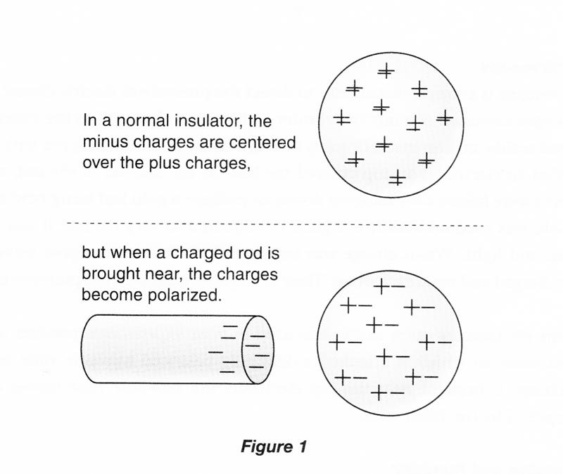
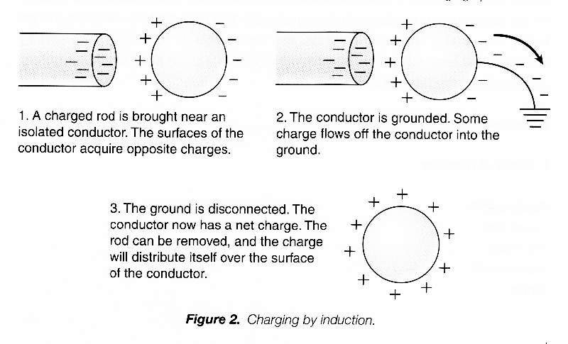
If the negative rod is brought near an isolated, neutral conductor, the conductor will also be polarized. In the conductor, electrons are free to move through the material, and some of them are repelled over to the opposite surface of the conductor, leaving the surface near the negative rod with a net positive charge. The conductor has been polarized, and will now be attracted to the charged rod.
Now if we connect a conducting wire or any other conducting material from the polarized conductor to the ground, we provide a “path” through which the electrons can move. Electrons will actually move along this path to the ground. If the wire or path is subsequently disconnected, the conductor as a whole is left with a net positive charge. The conductor has been charged without actually being touched with the charged rod, and its charge is opposite that of the rod. This procedure is called charging by induction.
THE ELECTROSCOPE
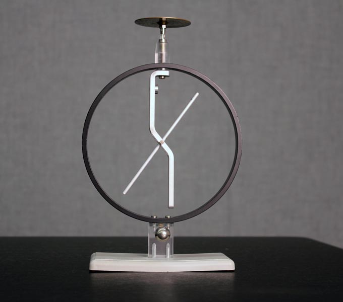
An electroscope is a simple instrument to detect the presence of electric charge. The old electroscopes consisted of a box or cylinder with a front glass wall so the experimenter could look inside, and an insulating top through which a conducting rod with a ball or disk (called an electrode) on top entered the box. At the bottom of the rod, very thin gold leaves were folded over hanging down, or perhaps a gold leaf hung next to a fixed vane. Gold was used because it is a good conductor and very ductile; it can be made very thin and light. When charge was transferred to the top, the gold leaves would become charged and repel each other. Their divergence indicated the presence of charge.
A modern electroscope such as the one used in your experiments consists of a fixed insulated vane, to which is attached a delicately balanced movable vane or needle. When charge is brought near the top electrode, the movable vane moves outward, being repelled by the fixed vane.
ELECTROSTATICS AND HUMIDITY
We are all familiar with the fact that cold, dry days are “hot” for electrostatics, and we get small shocks after walking across a rug and touching a door knob, or sliding across a car seat and touching the metal of the car door. If the humidity is fairly low on the day of your lab, the experiments will proceed easily. If the humidity is extremely low, as is often the case in Southern California, you will probably not escape the lab without a direct experience with electrostatics! If the humidity is high, as it is sometimes in the summer, the experiments are more difficult, and some may be impossible.
If the experiments are difficult on the first week of the electrostatics lab, they will be left up so you can try some of them with the Van de Graaff experiments in the following lab.
When the air is humid, a thin, invisible film of water forms on all surfaces, particularly on the surfaces of the insulators in the experiment. This film conducts away the charges before they have a chance to build up. You can ameliorate this effect somewhat by shining a heat lamp on the insulators in the apparatus. Do not bring the heat lamp too close, or the insulators will be melted.
EXPERIMENTS
EFFECT OF HUMIDITY
Equipment
Procedure
Record your observations in writing either on the computer (e.g., in Microsoft Word) or on your own paper. If writing by hand, write clearly, legibly, and neatly so that anyone, especially your TA, can read it easily. Start each observation with the section number and step number (e.g., I-2 for the step below). You do not need to repeat the question. Not all steps have observations to record.
Record in your notes the relative humidity in the room (from the wall meter) and the inside and outside temperature.
For this experiment, do not shine the flood lamp on the electroscope. Be prepared to start your timer. You may use the stopwatch function of your wristwatch.
Rub the lucite rod vigorously with the silk cloth. Use a little whipping motion at the end of the rubbing. Touch the lucite rod to the top of the electroscope. Move the rod along and around the top so you touch as much of its surface to the metal of the electroscope as possible. Since the rod is an insulator, charge will not flow from all parts of the rod onto the electroscope; you need to touch all parts (except where you are holding it) to the electroscope. Start your timer immediately after charging the electroscope.
Record the time it takes the electroscope needle to fall completely to 0°. Time up to five minutes, if necessary. If the needle has not fallen to 0° after five minutes, record an estimate of its angle at the five-minute mark. Typically, after charging, the needle might be at 80°.

If the electroscope needle falls to 0° in a few minutes, the heat lamp will help in the experiments below. If the needle falls to 0° in 15 seconds or so, as it does on some summer days, you will probably have difficulty completing the experiments, even with the help of the heat lamp. If this is the case, you can try again next week.
ATTRACTION AND REPULSION OF CHARGES
In this section, you will observe the characteristics of the two types of charges, and verify experimentally that opposite charges attract and like charges repel.
Equipment
Procedure
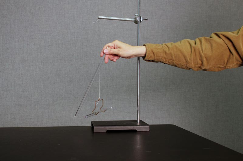
Charge one lucite rod by rubbing it vigorously with silk. Place the rod into the stirrup holder as shown in Figure 7.
Rub the second lucite rod with silk, and bring it close to the first rod. What happens? Record the observations in your notes.
Rub the rough plastic rod with cat's fur, and bring this rod near the lucite rod in the stirrup. Record your observations.
For reference purposes, according to the convention originally chosen by Benjamin Franklin, the lucite rods rubbed with silk become positively charged, and the rough plastic rods rubbed with cat's fur become negatively charged. Hard rubber rods, which are also commonly used, become negatively charged.
PITH BALLS
In this section, you will observe the induced polarization of a neutral insulator and the transfer of charge by contact.
Equipment

Procedure
(The heat lamp may help to minimize humidity near the pith balls.)
Touch the pith balls with your fingers to neutralize any charge.
Charge the lucite rod by rubbing it with silk.
Bring the lucite rod close to (but not touching) the pith balls. Observe and record what happens to the balls. Explain your results. (Refer to the theory section, if necessary.)
Touch the pith balls with your finger to discharge them. Recharge the lucite rod with silk.
Touch the pith balls with the lucite rod. (Sometimes it is necessary to touch different parts of the rod to the balls.) Then bring the rod near one of the balls. What happens? Record and explain your results.
Charge the rough plastic rod with cat's fur. How does the plastic rod affect the pith balls after they have been charged with the lucite rod? Record your results.
CHARGING BY INDUCTION
Equipment
Procedure
Charge the lucite rod by rubbing it with silk.
Bring the lucite rod near (but not touching) the top of the electroscope, so that the electroscope is deflected.
Remove the lucite rod. What happens? Record the results your notes. Use several sentences and perhaps a diagram or two to explain the behavior of the charges in the electroscope.
Bring the lucite rod near the electroscope again so that it is deflected. Hold the rod in this position, and briefly touch the top of the electroscope with your other finger. Keep the rod in position. What happens? Record the results in your notes.
Now remove the lucite rod. If you have done everything correctly, the electroscope should have a permanent deflection. Diagram in your notes what happened with the charges. (Refer to the theory section, if necessary.)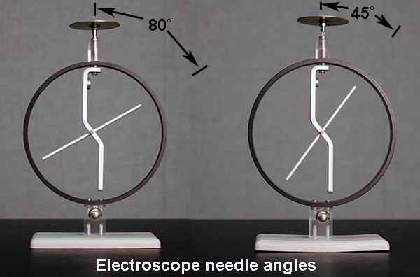
With the electroscope deflected as a result of the operations above, bring the charged lucite rod near the electroscope again. Remove the lucite rod, and bring a charged rough plastic rod near the electroscope. What happens in each case? Record the results in your notes.
ELECTROPHORUS
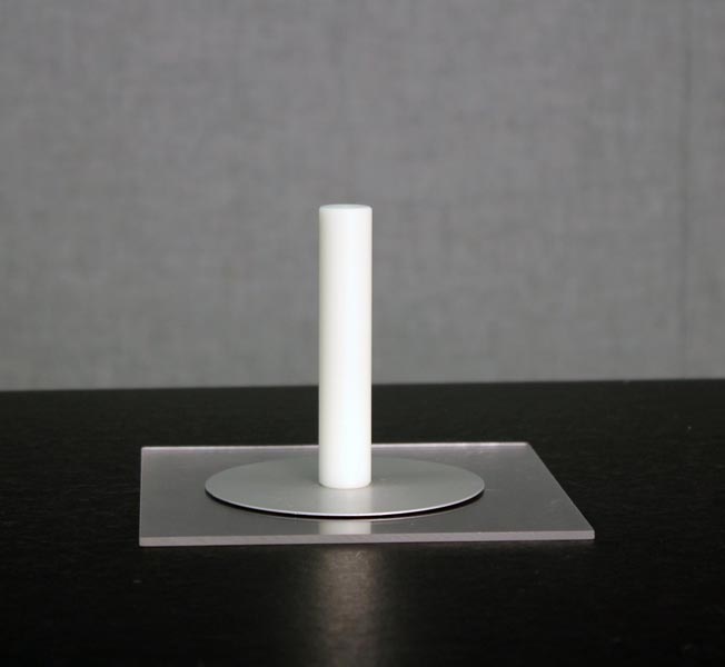
The electrophorus is a simple electrostatic induction device invented by Alessandro Volta around 1770. Volta characterized it as “an inexhaustible source of charge”. In its present form, the electrophorus consists of a lucite plate on which rests a flat metal plate with an insulating handle.
The lucite plate is positively charged by being rubbed with silk. Because lucite is an insulator, it remains charged until the charge leaks off slowly. The metal plate does not pick up this positive charge, even though it rests on the lucite. The plate actually makes contact with the lucite in only a few places; and because lucite is an insulator, charge does not transfer easily from it. Instead, when you touch the metal plate, electrons from your body (attracted by the positive lucite plate) flow onto the metal plate. Your body thus acts as an “electrical ground”. The metal plate is negatively charged by induction. Because the positive charge is not “used up”, the metal plate can be charged repeatedly by induction.
Equipment
Procedure
(The heat lamp shining on the equipment may improve its operation.)
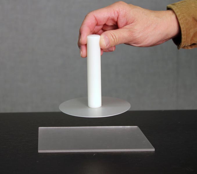
Charge the electrophorus lucite plate by rubbing it with silk. A whipping motion toward the end of the rubbing may help. Usually the lucite needs to be charged only once for the entire experiment.
Place the metal plate on the center of the lucite plate, and touch it with your finger. (You may feel a slight shock.)
Hold the metal plate by its insulating handle as far from the metal as possible. Bring the metal to within 2 cm of your knuckle, and then slowly closer until a (painless) spark jumps.
Recharge the metal plate by placing it back on the lucite, touching the lucite, and then lifting the plate off with its insulating handle. Bring it near your lab partner's knuckle.
Repeat the procedure until you have experienced several sparks. What is the average distance a spark will jump? Record this distance in your notes.
Recharge the metal plate, and bring it slowly near the top of the electroscope. Observe what happens with the electroscope needle.
Move the plate away from the electroscope, and record what happens with the electroscope needle. Is it still deflected? Why or why not?
Recharge the metal plate, and actually touch it to the top of the electroscope. Set the metal plate aside. Observe what happens with the electroscope needle. Is there any difference in the behavior of the needle compared to the results in procedure 6? If so, how do you account for the difference? Record this explanation in your notes.
Once again, recharge the metal plate. Hold one end of the neon tube with your fingers, and bring the metal plate slowly closer to the other end. Observe what happens with the neon tube. The induced current should create a brief flash of light. By grounding the end of the tube with your fingers, you are providing a pathway for the charges to move.
In this section, you charged the lucite plate by rubbing it at the beginning, and were then able to charge the metal plate repeatedly. Where does the charge on the metal plate come from? Where does the energy that makes the sparks and lights the tube come from? Comment in your notes.
COULOMB'S LAW
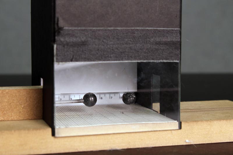
You will be testing the inverse \(r\)-squared dependence of Coulomb's Law with a very simple apparatus. There is a tall box containing a hanging pith ball covered with a conducting surface, and similar pith balls on sliding blocks. A mirrored scale permits you to determine the position of the balls. (The purpose of the closed box is to minimize the effects of air currents.)
The displacement \(d\) of the hanging ball from its equilibrium position depends on the electrical force \(F\) which repels it from the sliding ball. The force triangle of Figure 10 gives
\begin{eqnarray} \tan\phi &=& F/mg, \end{eqnarray}
while the physical triangle of the hanging ball gives
\begin{eqnarray} \sin\phi &=& d/L. \end{eqnarray}
If the angle \(\phi\) is small, then \(\tan\phi = \sin\phi\), and \(d\) is proportional to \(F\). Therefore, to demonstrate the inverse \(r\)-squared dependence of Coulomb's Law, we need to measure the displacement as a function of the separation between the centers of the balls.
The purpose of the mirror is to minimize parallax errors in reading the scale. For example, to measure to position of the front of the hanging ball, line up the front edge of the ball with its image. Your eye is now perpendicular to the scale, and you can read off the position. Figure 11 below shows the situation where your eye is still too high and to the right.
Equipment
Procedure
Take a moment to check to position of the hanging ball in your Coulomb apparatus. Look in through the side plastic window. The hanging ball should be at the same height as the sliding ball (i.e., the top of the mirrored scale should pass behind the center of the hanging pith ball, as in Figure 12 below). Lift off the top cover and look down on the ball. The hanging ball should be centered on a line with the sliding balls. If necessary, adjust carefully the fine threads that hold the hanging ball to position it properly.
Charge the metal plate of the electrophorus in the usual way by rubbing the plastic base with silk, placing the metal plate on the base, and touching it with your finger.
Lift off the metal plate by its insulating handle, and touch it carefully to the ball on the left sliding block.
Slide the block into the Coulomb apparatus without touching the sides of the box with the ball. Slide the block in until it is close to the hanging ball. The hanging ball will be attracted by polarization, as in Section III of this lab. After it touches the sliding ball, the hanging ball will pick up half the charge and be repelled away. Repeat the procedure if necessary, pushing the sliding ball up until it touches the hanging ball.
Recharge the sliding ball so it produces the maximum force, and experiment with pushing it toward the hanging ball. The hanging ball should be repelled strongly.
You are going to measure the displacement of the hanging ball. You do not need to measure the position of its center, but will record the position of its inside edge. Remove the sliding ball and record the equilibrium position of its inside edge that faces the sliding ball, which you will subtract from all the other measurements to determine the displacement \(d\).
Put the sliding ball in, and make trial measurements of the inside edge of the sliding ball and the inside edge of the hanging ball. The difference between these two measurements, plus the diameter of one of the balls, is the distance \(r\) between their centers. Practice taking measurements and compare your readings with those of your lab partner until you are sure you can do them accurately. Try to estimate measurements to 0.2 mm.
Take measurements, and record the diameter of the balls (by sighting on the scale).
Remove the sliding ball, and recheck the equilibrium position of the inside edge of the hanging ball.
You can record and graph data in Excel or by hand (although if you work by hand, you will lose the opportunity for 2 mills of additional credit below). Recharge the balls as in steps 1 – 4, and record a series of measurements of the inside edges of the balls. Move the sliding ball in steps of 0.5 cm for each new measurement.
Compute columns of displacements \(d\) (position of the hanging ball minus the equilibrium position) and the separations \(r\) (difference between the two recorded measurements plus the diameter of one ball).
Plot (by hand or with Excel) \(d\) versus \(1/r^2\). Is Coulomb's Law verified?
For an additional credit of 2 mills, use Excel to fit a power-law curve to the data. What is the exponent of the \(r\)-dependence of the force? (Theoretically, it should be −2.000, but what does your curve fit produce?)
For your records, you may print out your Excel file with a table and graph of your numerical observations and any other electronic files you have generated.
ADDITIONAL CREDIT (3 mills)
You can change the charge on the sliding ball by factors of two, by touching it to the other uncharged sliding ball (ground it with your finger first). The balls will share their charge, and half the charge will remain on the first ball (assuming the balls are the same size). This way, you can obtain charges on the first ball of \(Q\), \(Q/2\), \(Q/4\), and so forth.
Devise and execute an experiment to verify the dependence of the Coulomb force on the value of one of the charges. (That is, we want to show that the force is proportional to one of the charges.) The method is up to you; explain your plan and results in your notes. What should you plot against what? Does anything need to be held constant?
APPARATUS
INTRODUCTION
Measuring separately the electric charge (\(e\)) and the rest mass (\(m\)) of an electron is a difficult task because both quantities are extremely small (\(e\) = 1.60217733×10⁻¹⁹ coulombs, \(m\) = 9.1093897×10⁻³¹ kilograms). Fortunately, the ratio of these two fundamental constants can be determined easily and precisely from the radius of curvature of an electron beam traveling in a known magnetic field. An electron beam of a specified energy, and therefore a specified speed, may be produced conveniently in an \(e/m\) apparatus. The central piece of this apparatus is an evacuated electron-beam bulb with a special anode. A known current flows through a pair of Helmholtz coils and produces a magnetic field. The trajectory of the speeding electrons moving through the magnetic field is made visible by a small amount of mercury vapor.
THEORY
An electron moving in a uniform magnetic field travels in a helical path around the field lines. The electron's equation of motion is given by the Lorentz relation. If there is no electric field, then this relation can be written as
\begin{eqnarray} \textbf{F}_B &=& -e(\textbf{v}\times\textbf{B}), \label{eqn_1} \end{eqnarray}
where \(\textbf{F}_B\) is the magnetic force on the electron, \(-e\) = -1.6×10⁻¹⁹ coulombs is the electric charge of the electron, \(v\) is the velocity of the electron, and \(\textbf{B}\) is the magnetic field. In the special case where the electron moves in an orbit perpendicular to the magnetic field, the helical path becomes a circular path, and the magnitude of the magnetic force is
\begin{eqnarray} F_B &=& evB. \label{eqn_2} \end{eqnarray}
Recall from Physics 6A that an object traveling around a circle experiences a centripetal force. For an electron of mass m moving at speed \(v\) in a circle of radius \(R\), the magnitude of the centripetal force \(F_C\) is
\begin{eqnarray} F_C &=& mv^2/R. \label{eqn_3} \end{eqnarray}
Therefore,
\begin{eqnarray} evB &=& mv^2 /R, \end{eqnarray}
or
\begin{eqnarray} eB &=& mv/R. \label{eqn_4} \end{eqnarray}
The initial potential energy of the electrons in this experiment is \(eV\), where \(V\) is the accelerating voltage used in the electron-beam tube. After the electrons are accelerated through a voltage \(V\), this initial potential energy is converted into kinetic energy \((1/2)mv^2\). Since energy is conserved, it follows that
\begin{eqnarray} eV &=& (1/2)mv^2. \label{eqn_5} \end{eqnarray}
Combining Eqs. 4 and 5 yields
\begin{eqnarray} e/m &=& 2V/B^2 R^2. \label{eqn_6} \end{eqnarray}
THE \(e/m\) APPARATUS
The electron-beam bulb used in this experiment has a cathode that is heated indirectly, a collimating grid with a hole, and an anode with a hole.
Electrons leave the heated cathode and are attracted by the anode, which has a positive potential with respect to the cathode. Most electrons are stopped by the collimating grid and the anode. Those that are able to pass through the hole in the anode emerge from the back of the anode as a thin, monochromatic beam. The kinetic energy of the electrons in this beam is equal to the potential energy difference between the anode and the cathode.
To make the path of the electrons visible, we use the following method. The large evacuated glass bulb that houses the cathode and anode is spiked with a trace of mercury, enough to produce nearly saturated mercury vapor with a small pressure of approximately 1×10⁻³ mm Hg. (By comparison, recall that normal atmosphere pressure is approximately 760 mm Hg.) Occasionally an electron from the beam with a kinetic energy of about 300 eV collides with a mercury atom, causing the atom to become excited — a process that requires 10.4 eV of energy. The excited atom then decays quickly back to the ground state, emitting several photons in the process (including the one that has the characteristic blue color of mercury light). Thus, the blue halo in the glass bulb marks the path of the electrons. Note that the electron-beam tube, along with its socket, can be rotated nearly 90°.
The Helmholtz coils consist of a pair of identical circular coils of wire, each of radius \(r\), connected in series.
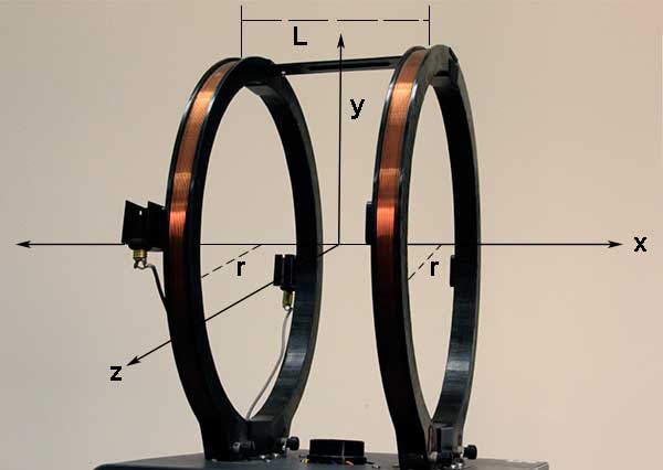
The distance between the coils is denoted \(L\). When \(L \ll r\), the coils produce a nearly uniform magnetic field in the space between them.
Along the axis of one thin coil with \(N\) turns at a distance \(x\) from the plane of the coil, the magnitude of the magnetic field \(B\) due to a current \(I\) is
\begin{eqnarray} B &=& \mu_0 r^2 N I/[2(r^2+x^2)^{3/2}]. \label{eqn_7} \end{eqnarray}
The direction of the magnetic field is perpendicular to the plane of the coil, and its unit is the tesla (T), with 1 tesla = 104 gauss. In SI units, the magnetic permeability μ0 of free space is
\begin{eqnarray} \mu_0 &=& 4\pi\times 10^{-7} \textrm{ Tm/A}. \end{eqnarray}
For a pair of identical parallel coils separated by a distance \(L\), the magnitude of the magnetic field at a point along the \(x\)-axis is
\begin{eqnarray} B &=& [\mu_0 r^2 NI/2] [ 1/(r^2+x^2)^{3/2} + 1/(r^2+(L-x)^2)^{3/2} ]. \label{eqn_8} \end{eqnarray}
When \(x = L/2 \), Eq. \eqref{eqn_8} gives
\begin{eqnarray} B &=& \mu_0 r^2 NI/(r^2+L^2/4)^{3/2}. \label{eqn_9} \end{eqnarray}
EQUIPMENT
The centerpiece of this experiment is the Kent \(e/m\) Experimental Apparatus Model TG-13, which consists of the electron-beam bulb (EBB) and a pair of Helmholtz coils (HC). There is also an illuminated ruler behind the EBB to facilitate the measurement of the electron-beam radius. The apparatus is fed by three external power sources. The accelerating voltage for the EBB is produced by a Heathkit Regulated Power Supply Model PS-4. A voltage of 150 – 300 V at a modest current of approximately 50 mA is required. This supply also provides the cathode heater power using a 6.3-V alternating current. The electric current and voltages are measured with two digital multimeters: the Triplett Multimeter Model 4000 and Simpson Digital Multimeter Model 464.
We use a GW Laboratory DC Power Supply Model GPS-1850 for the HC, which also supplies the voltage for the small light bulb of the illuminated scale. A large current of 1 – 2 A is needed, but a low voltage of 5 – 15 V is adequate. The \(e/m\) apparatus may be covered with a black cloth to reduce background light.
INITIAL SETUP
On the front panel of the \(e/m\) apparatus are jacks for the power and the voltmeter, two control knobs, and a switch. Starting from the left side of the panel, we have:
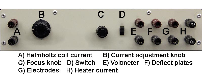
Two jacks (A) for the connection to the Helmholtz coils (HC) power supply. The current is measured by a multimeter connected in series with the power supply.
A current adjustment knob (B) for the HC. (The current can also be changed directly by a knob on the power supply.)
The focus knob (C), which allows sharpening of the electron beam by variation of the voltage on the grid of the EBB. The grid is internally connected and does not need a separate power supply.
A switch (D). This should be set in the “e/m Measure” position.
Two jacks (E) for the voltmeter, which measures the accelerating voltage.
Two jacks (F) for the deflection plates. (These are not used.)
Two jacks (G) for the high-voltage (~300 V) input to the electrodes of the electron gun.
Two jacks (H) for connecting the electron-gun heater to the power supply which can be 6.3-V DC or AC. (We use AC.)
Connect the EBB to the power supplies and multimeters (see the figure below).
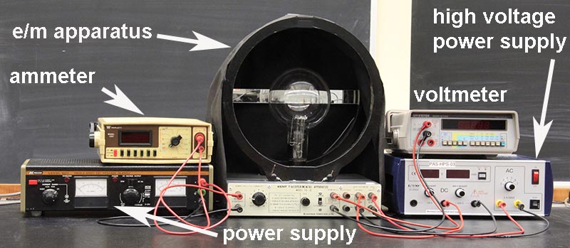
Use red cables for positive voltage and black cables for ground. To measure the HC current, make sure it passes through the Triplett multimeter in the current mode. (The HC power supply, the ammeter, and the HC are therefore connected in series.) Plug in the power supplies and the multimeters. Set the Triplett multimeter to the highest current scale, and put it in the DC-A mode. Connect the Simpson multimeter to the jacks labeled for the voltmeter (item E on the front panel of the EBB) set to the highest voltage scale, and put it in the DC-V mode.
PROCEDURE
Orient the Helmholtz coils (HC) so as to eliminate the influence of the Earth's magnetic field on the experiment. To do this, use a magnetic compass to determine the direction of the Earth's field, mark its direction on your work station with paper tape, and record its coordinates. Also measure and record the dip angle. Rotate the coils such that the plane of the HC lies in the plane of the Earth's magnetic field. With this orientation, the effect of the Earth's field on the HC is zero.
Connect the power supplies and multimeters to the \(e/m\) apparatus, as detailed in the previous section. Check that the polarities agree with the ones marked on the front panel of the apparatus.
Place the black cloth over the HC for easy observation of the electron beam. Turn on the heater supply, and allow two minutes for the filament to heat up. Apply 150 V to the anode, which should produce a visible beam. Turn on the current through the HC, and observe how the electron beam is bent and forms a circle.
Very carefully, rotate the glass bulb and observe the helical path of the electrons. Notice the direction of the helical axis.
Rotate the glass bulb such that the plane of the electron beam is exactly parallel to the plane of the HC. Using the focus control, obtain a well-defined beam. (You may also need to adjust the filament power to accomplish this.) If necessary, make a fine adjustment of the EBB's orientation so that the beam, after traveling a full circle, passes between the two metal struts which feed the power to the filament.
Set the HC current at a fixed value (e.g., 1 A). Measure \(R\) (the radius of the electron beam) for at least four settings of \(V\) (the accelerating voltage). Since \(e/m\) is proportional to \(1/R^2\), you should make an effort to measure \(R\) with small uncertainty. Use the mirror behind the EBB to minimize parallax. You may add a second ruler that is taped to the front of the HC.
Set the accelerating voltage at a fixed value (e.g., 200 V). Measure \(R\) for at least four settings of \(I\) (the HC current).
The manufacturer of the \(e/m\) apparatus did not supply the number of windings, \(N\), of the HC. On the front panel of the EBB stand, it is stated that \(B\) = (7.8 \(I\)) gauss, but no uncertainty is given. To determine the magnitude of the magnetic field, you will use a calibrated magnetometer (Bell 620 Gaussmeter) based on a calibrated Hall Probe.
Your TA will remove the EBB. Install the Hall-Probe holder in the HC. Calibrate the magnitude of the magnetic field \(B\) in the center of the HC for the four values of the current \(I\), including two different scale settings. Plot \(B\) as a function of \(I\). Note that the error in \(e/m\) is proportional to \(1/B^2\) (see Eq. \eqref{eqn_6}). Use the \(B\) versus \(I\) graph to determine the magnetic field for each value of the current.
Plot \(V\) as a function of \(R^2\) (the data in step 6), and use the slope of the graph to determine the ratio \(e/m\) with the help of Eq. \eqref{eqn_6}.
Plot \(I^2\) as a function of \(1/R^2\) (the data in step 7), and use the slope of the graph to determine the ratio \(e/m\) with the help of Eq. \eqref{eqn_6}.
Compute the ratio \(e/m\) using the “accepted” values provided in the “Introduction” section of this experiment, and compare it with your measured ratios from parts 8 and 9.
DETERMINATION OF THE ACCELERATION VOLTAGE
The absolute calibration of a voltage meter is a very difficult task. Traditionally, one uses standard cells which are stored at the National Calibration Laboratory in various countries. A new method depends on the so-called Josephson effect. We will assume that the multimeters have been calibrated sufficiently well. However, we should compare the voltage readings of the two multimeters to estimate the minimal value for the absolute error.
DATA
Coordinates of Earth's magnetic field =
Dip angle =
\(V\) (Trial 1) =
\(R\) (Trial 1) =
\(V\) (Trial 2) =
\(R\) (Trial 2) =
\(V\) (Trial 3) =
\(R\) (Trial 3) =
\(V\) (Trial 4) =
\(R\) (Trial 4) =
\(I\) (Trial 1) =
\(R\) (Trial 1) =
\(I\) (Trial 2) =
\(R\) (Trial 2) =
\(I\) (Trial 3) =
\(R\) (Trial 3) =
\(I\) (Trial 4) =
\(R\) (Trial 4) =
\(B\) (Trial 1) =
\(B\) (Trial 2) =
\(B\) (Trial 3) =
\(B\) (Trial 4) =
Plot the graph of \(B\) as a function of \(I\) using one sheet of graph paper at the end of this workbook. Remember to label the axes and title the graph.
Plot the graph of \(V\) as a function of \(R^2\) using one sheet of graph paper at the end of this workbook. Remember to label the axes and title the graph.
Slope of graph =
\(e/m\) =
Plot the graph of \(I^2\) as a function of \(1/R^2\) using one sheet of graph paper at the end of this workbook. Remember to label the axes and title the graph.
Slope of graph =
\(e/m\) =
\(e/m\) (computed from accepted values provided in “Introduction”) =
Percentage difference between experimental and accepted \(e/m\) from part 8 =
Percentage difference between experimental and accepted \(e/m\) from part 9 =
Links:
[1] https://demoweb.physics.ucla.edu/sites/default/files/Physics6B_Exp1.pdf
[2] https://demoweb.physics.ucla.edu/sites/default/files/Physics6B_Exp2.pdf
[3] https://demoweb.physics.ucla.edu/sites/default/files/Physics6B_Exp4.pdf
[4] https://demoweb.physics.ucla.edu/sites/default/files/Physics6B_Exp5.pdf