Instructional Resource Lab
Experiment 6 - The Photoelectric Effect
APPARATUS
- Photodiode with amplifier
- Batteries to operate amplifier and provide reverse voltage
- Digital voltmeter to read reverse voltage
- Source of monochromatic light beams to irradiate photocathode
- Neutral filter to vary light intensity
INTRODUCTION
The energy quantization of electromagnetic radiation in general, and of light in particular, is expressed in the famous relation
\begin{eqnarray} E &=& hf, \label{eqn_1} \end{eqnarray}
where \(E\) is the energy of the radiation, \(f\) is its frequency, and \(h\) is Planck's constant (6.63×10⁻³⁴ Js). The notion of light quantization was first introduced by Planck. Its validity is based on solid experimental evidence, most notably the photoelectric effect. The basic physical process underlying this effect is the emission of electrons in metals exposed to light. There are four aspects of photoelectron emission which conflict with the classical view that the instantaneous intensity of electromagnetic radiation is given by the Poynting vector \(\textbf{S}\):
\begin{eqnarray} \textbf{S} &=& (\textbf{E}\times\textbf{B})/\mu_0, \label{eqn_2} \end{eqnarray}
with \(\textbf{E}\) and \(\textbf{B}\) the electric and magnetic fields of the radiation, respectively, and μ0 (4π×10-7 Tm/A) the permeability of free space. Specifically:
-
No photoelectrons are emitted from the metal when the incident light is below a minimum frequency, regardless of its intensity. (The value of the minimum frequency is unique to each metal.)
-
Photoelectrons are emitted from the metal when the incident light is above a threshold frequency. The kinetic energy of the emitted photoelectrons increases with the frequency of the light.
-
The number of emitted photoelectrons increases with the intensity of the incident light. However, the kinetic energy of these electrons is independent of the light intensity.
-
Photoemission is effectively instantaneous.
THEORY
Consider the conduction electrons in a metal to be bound in a well-defined potential. The energy required to release an electron is called the work function \(W_0\) of the metal. In the classical model, a photoelectron could be released if the incident light had sufficient intensity. However, Eq. \eqref{eqn_1} requires that the light exceed a threshold frequency \(f_{\textrm{t}}\) for an electron to be emitted. If \(f > f_{\textrm{t}}\), then a single light quantum (called a photon) of energy \(E = hf\) is sufficient to liberate an electron, and any residual energy carried by the photon is converted into the kinetic energy of the electron. Thus, from energy conservation, \(E = W_0 + K\), or
\begin{eqnarray} K &=& (1/2)mv^2 = E - W_0 = hf - W_0. \label{eqn_3} \end{eqnarray}
When the incident light intensity is increased, more photons are available for the release of electrons, and the magnitude of the photoelectric current increases. From Eq. \eqref{eqn_3}, we see that the kinetic energy of the electrons is independent of the light intensity and depends only on the frequency.
The photoelectric current in a typical setup is extremely small, and making a precise measurement is difficult. Normally the electrons will reach the anode of the photodiode, and their number can be measured from the (minute) anode current. However, we can apply a reverse voltage to the anode; this reverse voltage repels the electrons and prevents them from reaching the anode. The minimum required voltage is called the stopping potential \(V_{\textrm{s}}\), and the “stopping energy” of each electron is therefore \(eV_{\textrm{s}}\). Thus,
\begin{eqnarray} eV_{\textrm{s}} &=& hf - W_0, \label{eqn_4} \end{eqnarray}
or
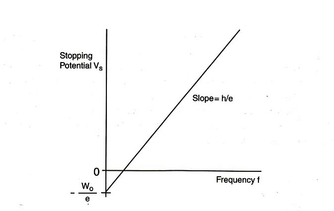
\begin{eqnarray} V_{\textrm{s}} &=& (h/e)f - W_0/e. \label{eqn_5} \end{eqnarray}
Eq. \eqref{eqn_5} shows a linear relationship between the stopping potential \(V_{\textrm{s}}\) and the light frequency \(f\), with slope \(h/e\) and vertical intercept \(-W_0/e\). If the value of the electron charge \(e\) is known, then this equation provides a good method for determining Planck's constant \(h\). In this experiment, we will measure the stopping potential with modern electronics.
THE PHOTODIODE AND ITS READOUT
The central element of the apparatus is the photodiode tube. The diode has a window which allows light to enter, and the cathode is a clean metal surface. To prevent the collision of electrons with air molecules, the diode tube is evacuated.
The photodiode and its associated electronics have a small “capacitance” and develop a voltage as they become charged by the emitted electrons. When the voltage across this “capacitor” reaches the stopping potential of the cathode, the voltage difference between the cathode and anode (which is equal to the stopping potential) stabilizes.
To measure the stopping potential, we use a very sensitive amplifier which has an input impedance larger than 1013 ohms. The amplifier enables us to investigate the minuscule number of photoelectrons that are produced.
It would take considerable time to discharge the anode at the completion of a measurement by the usual high-leakage resistance of the circuit components, as the input impedance of the amplifier is very high. To speed up this process, a shorting switch is provided; it is labeled “Push to Zero”. The amplifier output will not stay at 0 volts very long after the switch is released. However, the anode output does stabilize once the photoelectrons charge it up.
There are two 9-volt batteries already installed in the photodiode housing. To check the batteries, you can use a voltmeter to measure the voltage between the output ground terminal and each battery test terminal. The battery test points are located on the side panel. You should replace the batteries if the voltage is less than 6 volts.
THE MONOCHROMATIC LIGHT BEAMS
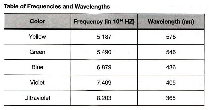
This experiment requires the use of several different monochromatic light beams, which can be obtained from the spectral lines that make up the radiation produced by excited mercury atoms. The light is formed by an electrical discharge in a thin glass tube containing mercury vapor, and harmful ultraviolet components are filtered out by the glass envelope. Mercury light has five narrow spectral lines in the visible region — yellow, green, blue, violet, and ultraviolet — which can be separated spatially by the process of diffraction. For this purpose, we use a high-quality diffraction grating with 6000 lines per centimeter. The desired wavelength is selected with the aid of a collimator, while the intensity can be varied with a set of neutral density filters. A color filter at the entrance of the photodiode is used to minimize room light.
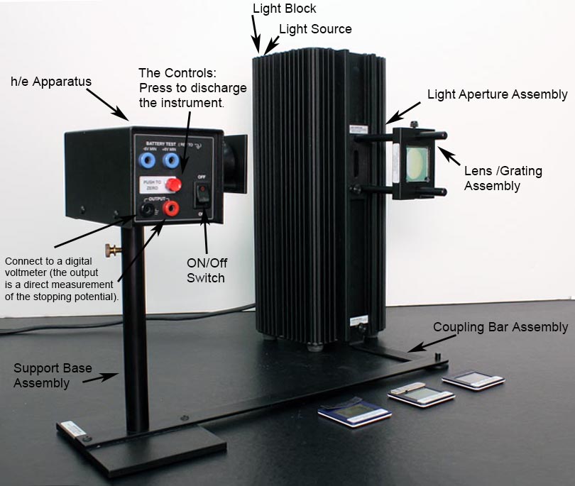
The equipment consists of a mercury vapor light housed in a sturdy metal box, which also holds the transformer for the high voltage. The transformer is fed by a 115-volt power source from an ordinary wall outlet. In order to prevent the possibility of getting an electric shock from the high voltage, do not remove the cover from the unit when it is plugged in.
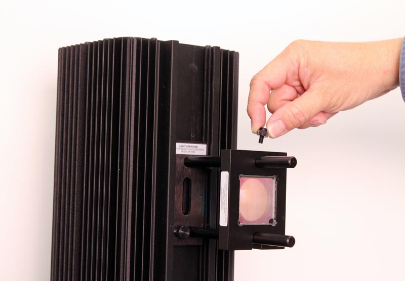
To facilitate mounting of the filters, the light box is equipped with rails on the front panel. The optical components include a fixed slit (called a light aperture) which is mounted over the output hole in the front cover of the light box. A lens focuses the aperture on the photodiode window. The diffraction grating is mounted on the same frame that holds the lens, which simplifies the setup somewhat. A “blazed” grating, which has a preferred orientation for maximal light transmission and is not fully symmetric, is used. Turn the grating around to verify that you have the optimal orientation.
The variable transmission filter consists of computer-generated patterns of dots and lines that vary the intensity of the incident light. The relative transmission percentages are 100%, 80%, 60%, 40%, and 20%.
INITIAL SETUP
-
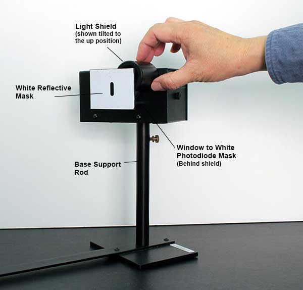
Your apparatus should be set up approximately like the figure above. Turn on the mercury lamp using the switch on the back of the light box. Swing the \(h/e\) apparatus box around on its arm, and you should see at various positions, yellow green, and several blue spectral lines on its front reflective mask. Notice that on one side of the imaginary “front-on” perpendicular line from the mercury lamp, the spectral lines are brighter than the similar lines from the other side. This is because the grating is “blazed”. In you experiments, use the first order spectrum on the side with the brighter lines.
-
Your apparatus should already be approximately aligned from previous experiments, but make the following alignment checks. Ask you TA for assistance if necessary.
-
Check the alignment of the mercury source and the aperture by looking at the light shining on the back of the grating. If necessary, adjust the back plate of the light-aperture assembly by loosening the two retaining screws and moving the plate to the left or right until the light shines directly on the center of the grating.
-
With the bright colored lines on the front reflective mask, adjust the lens/grating assembly on the mercury lamp light box until the lines are focused as sharply as possible.
-
Roll the round light shield (between the white screen and the photodiode housing) out of the way to view the photodiode window inside the housing. The phototube has a small square window for light to enter. When a spectral line is centered on the front mask, it should also be centered on this window. If not, rotate the housing until the image of the aperture is centered on the window, and fasten the housing. Return the round shield back into position to block stray light.
-
-
Connect the digital voltmeter (DVM) to the “Output” terminals of the photodiode. Select the 2 V or 20 V range on the meter.
-
Press the “Push to Zero” button on the side panel of the photodiode housing to short out any accumulated charge on the electronics. Note that the output will shift in the absence of light on the photodiode.
-
Record the photodiode output voltage on the DVM. This voltage is a direct measure of the stopping potential.
-
Use the green and yellow filters for the green and yellow mercury light. These filters block higher frequencies and eliminate ambient room light. In higher diffraction orders, they also block the ultraviolet light that falls on top of the yellow and green lines.
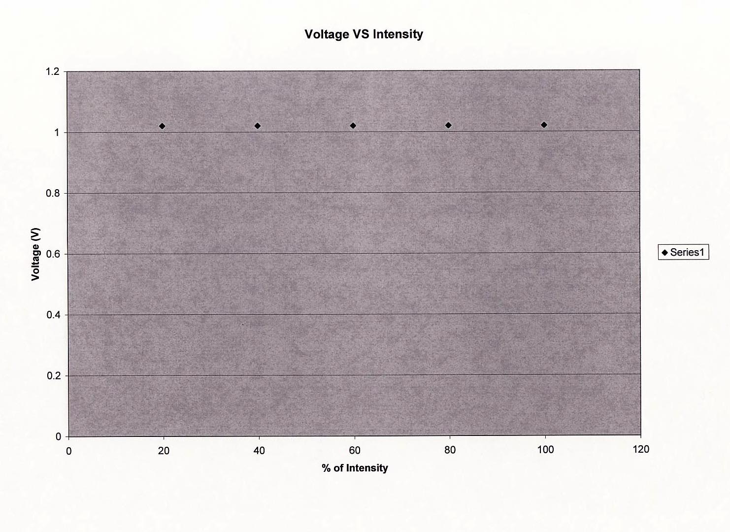
PROCEDURE PART 1: DEPENDENCE OF THE STOPPING POTENTIAL ON THE INTENSITY OF LIGHT
-
Adjust the angle of the photodiode-housing assembly so that the green line falls on the window of the photodiode.
-
Install the green filter and the round light shield.
-
Install the variable transmission filter on the collimator over the green filter such that the light passes through the section marked 100%. Record the photodiode output voltage reading on the DVM. Also determine the approximate recharge time after the discharge button has been pressed and released.
-
Repeat steps 1 – 3 for the other four transmission percentages, as well as for the ultraviolet light in second order.
-
Plot a graph of the stopping potential as a function of intensity.
PROCEDURE PART 2: DEPENDENCE OF THE STOPPING POTENTIAL ON THE FREQUENCY OF LIGHT
You can see five colors in the mercury light spectrum. The diffraction grating has two usable orders for deflection on one side of the center.
-
Adjust the photodiode-housing assembly so that only one color from the first-order diffraction pattern on one side of the center falls on the collimator.
-
For each color in the first order, record the photodiode output voltage reading on the DVM.
-
For each color in the second order, record the photodiode output voltage reading on the DVM.
-
Plot a graph of the stopping potential as a function of frequency, and determine the slope and the \(y\)-intercept of the graph. From this data, calculate \(W_0\) and \(h\). Compare this value of \(h\) with that provided in the “Introduction” section of this experiment.
DATA
Procedure Part 1:
-
Photodiode output voltage reading for 100% transmission =
Approximate recharge time for 100% transmission =
-
Photodiode output voltage reading for 80% transmission =
Approximate recharge time for 80% transmission =
Photodiode output voltage reading for 60% transmission =
Approximate recharge time for 60% transmission =
Photodiode output voltage reading for 40% transmission =
Approximate recharge time for 40% transmission =
Photodiode output voltage reading for 20% transmission =
Approximate recharge time for 20% transmission =
Photodiode output voltage reading for ultraviolet light =
Approximate recharge time for ultraviolet light =
-
Plot the graph of stopping potential as a function of intensity using one sheet of graph paper at the end of this workbook. Remember to label the axes and title the graph.
Procedure Part 2:
-
First-order diffraction pattern on one side of the center:
Photodiode output voltage reading for yellow light =
Photodiode output voltage reading for green light =
Photodiode output voltage reading for blue light =
Photodiode output voltage reading for violet light =
Photodiode output voltage reading for ultraviolet light =
-
Second-order diffraction pattern on the other side of the center:
Photodiode output voltage reading for yellow light =
Photodiode output voltage reading for green light =
Photodiode output voltage reading for blue light =
Photodiode output voltage reading for violet light =
Photodiode output voltage reading for ultraviolet light =
-
Plot the graph of stopping potential as a function of frequency using one sheet of graph paper at the end of this workbook. Remember to label the axes and title the graph.
Slope of graph =
\(y\)-intercept of graph =
\(W_0\) =
\(h\) =
Percentage difference between experimental and accepted values of \(h\) =