
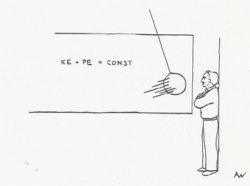
A Set of First Day Demos with Audience Appeal and Discussion
Some instructors like to give a "magic show" on the first day of class to illustrate some of the physics that will be covered during the quarter. Examples of mechanics demos with audience appeal are (see entry further in catalog for illustration and more description):
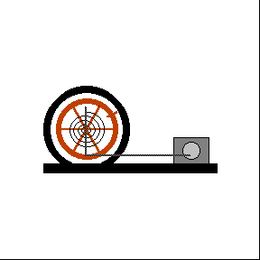
Unidentified Rolling Objects [1]
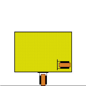
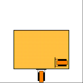
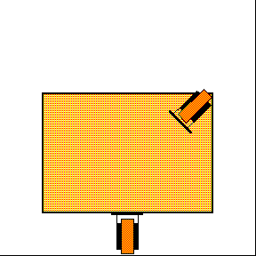
Turntable and Bicycle Wheel [5]
Another suggestion for the first day of class is to do a set of demos that review a little high school physics and lead into the subjects to be covered in the first two weeks. Here is a sample scenario:
Start with Drop Two Balls [6]. Ask your students, "If I drop this steel ball and this wooden ball simultaneously from the same height, which will hit the ground first?" You will be surprised at the various answers, even from a Physics 8A class. Solicit explanations from several different students of their reasoning; this will give you an idea of the level of the class. If most of the students claim the balls will hit the ground at the same time ask, "What if I drop this ball and this sheet of paper?" This can then lead into a discussion of the effects of air resistance and what factors influence it, like the area fronting the wind. Lester Hirsch suggests: Borrow the two sheets of paper from two different students. Tell them not to tear the pages out of their notebooks; you are going to return the pages. Crumple one up into a ball and drop it simultaneously with a flat sheet. Here we have isolated the effect of air resistance by dropping two objects with the same mass, but different shapes. After the demonstration hand the flat sheet back to the first student, and carefully smooth out the crumpled sheet and hand it back to the second student. When he makes a face, tell the class that conservation has to start somewhere, and that he has to be the one this time!
To make this demonstration somewhat more quantitative, you may wish project a slide of a wooden ball, a steel ball, and a ping-pong ball falling, photographed at 1/20 sec. intervals. (See Three Balls Falling [7])
The Guinea and Feather Tube [8] might well be used in this discussion also.
If you establish in a high level class that all of the students are pretty clear on the concepts of equal gravitational acceleration for different masses and effect of air resistance, try the following, "According to Newton's Third Law, what force is equal and opposite the weight of this steel ball I am holding in my hand?" You will get a variety of different answers to this question. After the discussion establishes that the third law pair to the weight of the ball acts on the entire planet Earth, ask, "So, according to Newton's Third Law, the steel ball exerts a force equal to its weight on planet Earth. As the two balls fall, doesn't the steel ball pull the Earth over towards it more than the wooden ball, so the steel ball must really strike the Earth first, even if we neglect air resistance?"
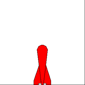
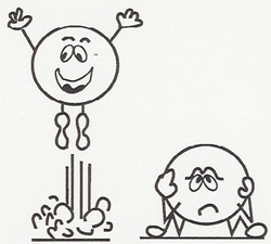
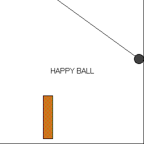
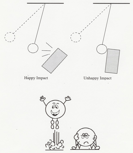
As a final first-day demonstration, drop the "happy" and "unhappy" balls to show that objects that look identical may have very different physical properties.
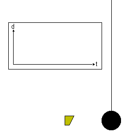
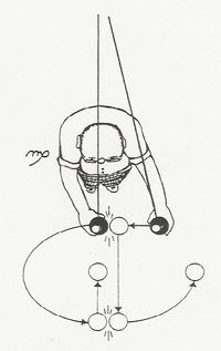
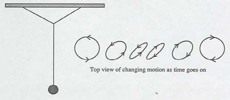
This very simple demonstration of a pendulum swinging above two magnets illustrates that Newton's laws do not always lead to predictable orderly motion. The pendulum bob is released from various initial positions, and it eventually comes to rest over one of the magnets, usually after undergoing complex irregular motion, often jumping from one magnet to the other. If you could accurately mark the release points for which the bob winds up over magnet one, you would find a "fractal" curve which is complex under any magnification. Points infinitesimally close to a point for which the bob winds up over magnet one will lead to the bob finishing over magnet two. It is not really practical to develop this curve in class, but the chaotic irregular motion of the bob is striking. This demo is suggested in Turning the World Inside Out by Robert Ehrlich (Princeton University Press 1990).
There is also a compound pendulum which shows chaotic motion (see Compound Chaotic Pendulum [9]).
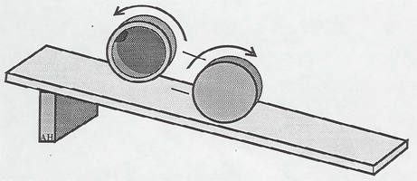
a. Unpredictable discs
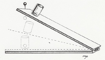
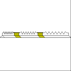
Ask the class which of two identical looking discs will roll down an inclined plane the fastest. Most students will say they will roll equally, but one rolls down, and the other rolls up the inclined plane!
Also two identical looking cylinders roll down at different rates.
b. Premature stopping of cylinder
A cylinder rolls half-way down an inclined plane and then stops.
c. Reversing cylinder
A cylinder rolls down the inclined plane, and then rolls back up!
d. Unpredictable Pendulum
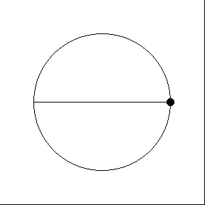
Pendulum swings irregularly around, deflected by a hidden magnet.
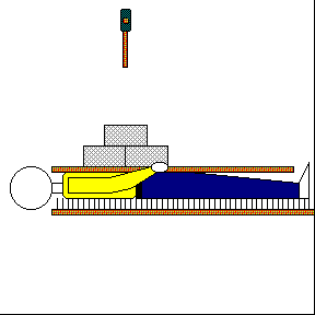
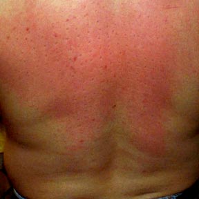
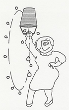
A "volunteer" removes glasses and jewelry and lies on a bed of 4000 nails. A male volunteer can take off his shirt so that his bare skin is against the nails. A plywood sheet is placed over him and several concrete blocks piled on top. The demonstrator then smashes the blocks with a sledge hammer.
Several physics principles are involved here. The force from any one nail is reduced by spreading the weight over many nails. The inertia of the blocks partially protects the person below from the force of impact. The smashing of the blocks absorbs much of the energy of the blow.
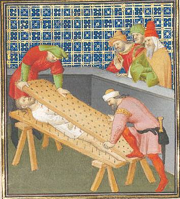
Using too few nails in this demo was a form of torture. In the illustration below Roman consul Marcus Atilius Regulus is tortured to death by Carthaginians in about 255 BC. The illustration was painted in about 1415 in Paris.
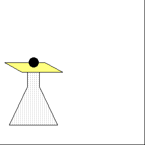
A card with a small ball is placed over a flask. When the card is flicked away with the finger, the ball will not move with it but will fall straight down into the flask.
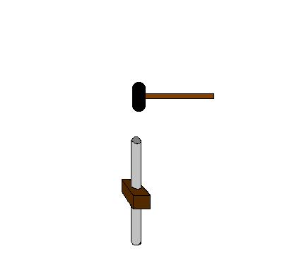
A PVC tube goes through the center of a wooden block, which is free to move along the tube after overcoming some amount of friction. As you hammer down on the tube while holding on to it with one hand the block moves up along the tube.
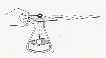
This is a dramatic demonstration of inertia. A metal hoop of spring steel is balanced on the mouth of a flask, and a piece of chalk is balanced on the hoop, directly over the mouth of the flask. The object is to snatch the hoop away so the chalk falls into the flask. Tell your audience that this is a difficult demonstration and you need a couple of practice shots first. In your "practice shots" grab the hoop by its leading edge so the top is compressed upward ejecting the chalk wildly into the air. After telling the audience you are now ready to try it for real, grab the hoop by its trailing edge so its top is pulled out from under the chalk, dropping the chalk neatly into the flask! (From The Physics Teacher, Feb. 1982).
A massive ball is suspended by a string with a string below. Using a rod, the demonstrator pulls or jerks down on the lower string. A steady pull always breaks the upper string; a jerk always breaks the lower string.
 With a Jerk |
 Pulling Steadily |
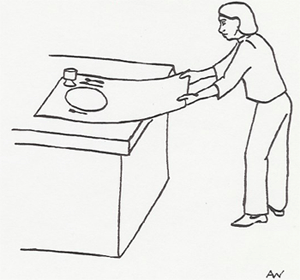
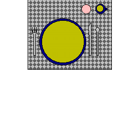
Bring down the house with this old favorite. A plate and silverware are laid out in a place setting on a sheet of paper. A glass of water, beer, or wine adds impact. With a swift jerk the demonstrator pulls out the paper, leaving the place setting intact.
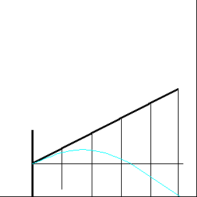
Which way will the Moon go if the earth's gravity were suddenly switched off? The Pie Plate demo gives a good analogy. Spin a ball around the inside rim of the plate. The inward force of the rim keeps the ball in circular motion. But when the rim ends, the ball flies off in a straight line, obeying Newton’s First Law.
|
| A Scientific American article ("Intuitive Physics" by Michael McCloskey, Scientific American, April 1983) discusses how students, when asked which way the ball will go upon leaving the pie plate before having taken a course in physics, will usually answer that the ball will continue to curve around. Of course, right after taking physics the students (at least the ones that pass the course!) know that the ball moves off in a straight line. But a few years after the course, the ball starts to curve again! The students were enlightened; they knew the truth, but then they fell back into darkness! (The same article discusses several other misconceptions of motion you may wish to discuss with your students.) |
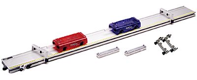
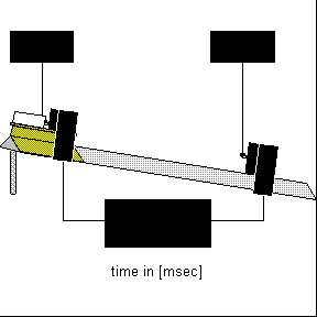
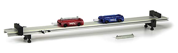
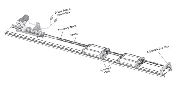
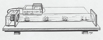
In addition to its usefulness in qualitative demonstrations of linear motion and collisions the dynamics track shown below can be used in conjunction with Data Studio and a motion sensor to measure and plot the position, velocity and acceleration of a Pasco cart as a function of time.

In the following Data Studio experiment for constant linear motion, the Pasco track was propped up slightly on one end with adequate metal slugs to compensate for friction. Then the cart was given a slight push to achieve constant velocity. The motion sensor was used to measure and graph the cart's position as a function of time. The graph shows that the position changes linearly as a function of time. A linear fit to the position vs. time curve gives the slope to be 0.45 m/s. This constant value corresponds to the average and instantaneous velocities for this experiment. Furthermore, it is within experimental error of the mean of the velocity vs. time curve (0.46 m/s). Taking the slope of the velocity vs. time curve, we find that it is zero and therefore have zero acceleration -- also demonstrated experimentally.
Various other linear motion demonstrations can be performed with the dynamics track which also allow for quantitative analysis. The track may be set up with two electronic timers that measure the time it takes a 10 cm flag mounted on a cart to pass in front of an infrared sensor. Thus, these timers are measuring (the reciprocal of) the velocity of the carts.
Another timer is available to measure the elapsed time for a cart to cover a given distance.
a. Newton's 1st law A cart is set moving along the track past the two velocity times. The track can be set up to compensate for friction such that the velocity of the glider remains essentially constant.

b. Gravitational Acceleration If one end of the track is raised slightly, measurements can be taken of a cart accelerating down the track.

c. Newton's 2nd Law A ribbon is attached to a cart and passed over a frictionless pulley to a falling weight. By varying the mass of the weight and the cart, measurements can be taken verifying Newton's 2nd Law.
d. Collisions and Explosions Elastic and ineleastic collisions between carts can be demonstrated as one end of the carts are equipped with magnets and the other end with Velcro. A moving cart collides elastically with a stationary cart of equal mass using the magnetic ends. The originally stationary cart moves away with all the velocity. Completely inelastic collisions result by colliding the Velcro ends of the carts. A carts velocity is measured before and after it has collided inelastically with another cart of equal mass. It is demonstrated that the velocity of the two carts after the collision is half the initial value.
|
Elastic Collision |
Inelastic Collision |
|---|---|
 |
 |
Explosions are demonstrated by touching the ends of two carts together and releasing an internal plunger from one of the carts.
|
Explosion |
|---|
 |
All of the above demos may also be demonstrated with the air track at the instructor's request. The air track has an advantage over the dynamics track in that there is less friction associated with it. However, the air track has a draw-back in that it is much noisier than the dynamics track and in a lecture setting it is difficult for the instructor to be heard.
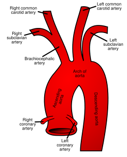
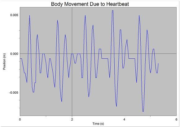
A person lies down on a flat board set on rollers. A laser beam is directed at a tiny mirror positioned on one of the rollers. The laser beam is projected onto the ceiling or wall. The beating of the person's heart causes a slight movement in the body as indicated by the laser. This upward movement of the body is due to the 3rd Law reaction force of the blood being pumped to the lower body. The left ventricle of the heart squeezes blood upward into the aorta shown below. At the peak of the contraction, about 80 grams of blood is moving upward at 30 cm/s. The aorta does a U-turn forcing most of the blood to flow down to the lower body. The aorta and body force the blood down and in turn the body is forced up. The amount is too small to be seen by eye but can be seen when "amplified" by the laser-mirror arrangement used in the demonstration. It can also be seen when standing quietly on a weight scale if the scale is sensitive enough and the vibration is not damped by the scale mechanism. Your weight decreases slightly when the blood slams into the top of the aorta.
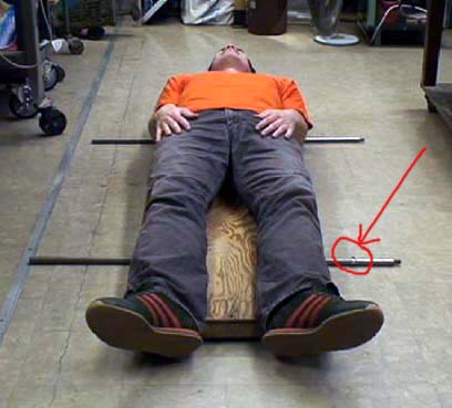
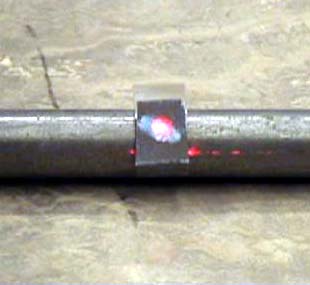
A video of the movement of the body as detected by the laser-mirror setup as well as a graph tracing the motion are provided below.
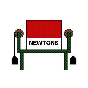
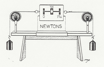
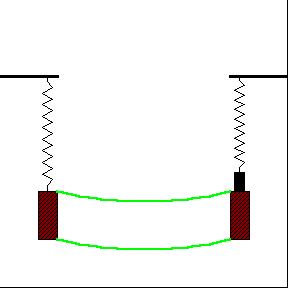
A 1 kg mass weighs 9.8 N as checked by a spring scale. Two 1 kg masses are hooked on the ends of a string which is passed over a pair of pulleys, and the spring scale is placed in the center of the string to measure the tension as shown. The scale is covered with a cloth to hide its reading, and the class is then asked to predict whether the scale will read 0, 9.8, or 19.6 N.
Water Rocket — A toy rocket is loaded with water and compressed air and shot across the room. It can also be fired with air only (no water in it) to show the difference.
C02 rocket — A rod mounted on the end of a shaft is free to turn about the shaft's axis. At the end of the rod is a C02 cartridge. When the cartridge is punctured, the escaping gasses propel the rod with considerable speed.
Hero's engine — spins by the reaction force of escaping steam.
The dynamics track cart has a sail and a battery operated propeller; both are removable. If the propeller is removed and held so it blows against the sail, the cart will roll to the left. If the sail is removed and the propeller mounted alone, the cart will accelerate to the right. If both the sail and the propeller are mounted, the instructor can ask the students which way the cart will roll.
From S.R. Smith and J.D. Wilson, Phys. Teacher, Apr. 72, pp 208.

Note: The above demos may also be demonstrated with the air track at the instructor's request. The air track has an advantage over the dynamics track in that there is less friction associated with it. However, the air track has a draw-back in that it is much nosier than the dynamics track and in a lecture setting it is difficult for the instructor to be heard.
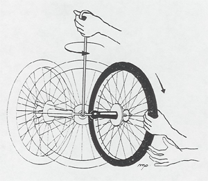
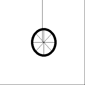
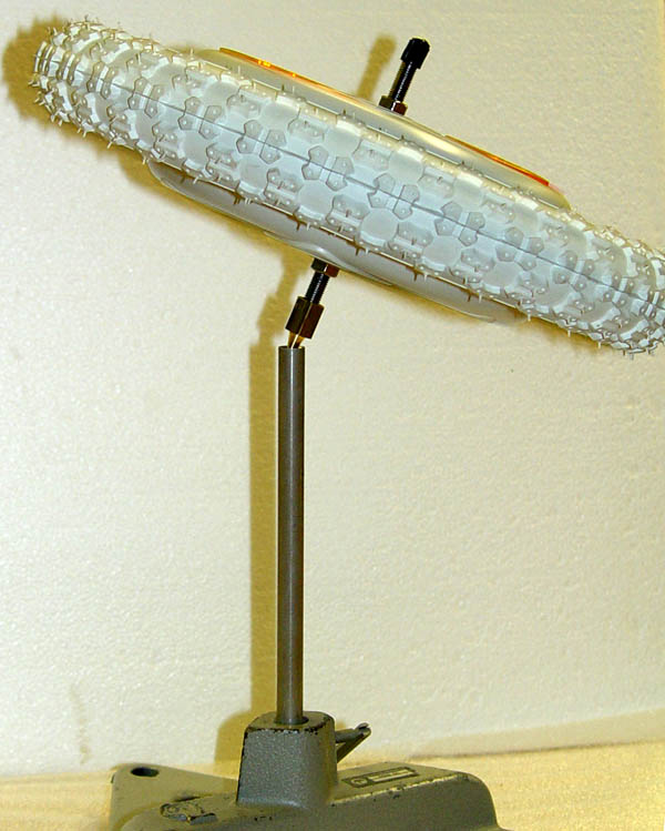
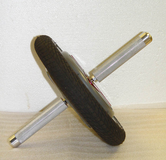
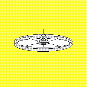
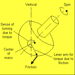
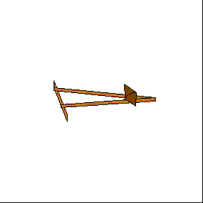
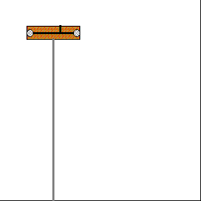
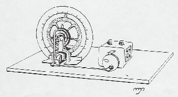
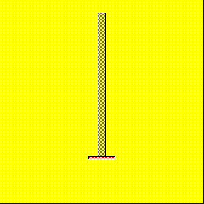
A spinning bicycle wheel suspended by a rope from one end of its axle makes an impressive gyro. A skillful demonstrator can start the wheel precessing smoothly so that the axle remains horizontal.
Other gyros available:
Two standard gyros spun up with a small motor.

Fully gimboled gyro to demonstrate maintenance of axis of rotation and inertial guidence.
Gyrowheel a small bicycle wheel with a motorized gyro inside, can be used on the rotating platform or as a precessing top
Cenco top a large bicycle wheel sized gyro, the center of mass of which can be varied above and below the point of support.
Massive air bearing ball gyro operates with so little friction that the rate of rotation can be made smaller than the rate of precession. Measurements can be taken to check the relationship between the angular velocities of rotation and precession.
Various tops are available including a "tippy top" consisting of a hemisphere with an axle shaft above. When set spinning on the hemisphere, the top will flip upside down and spin on its axle.
A "perpetual motion" top spins indefinitely with no apparent external energy source.
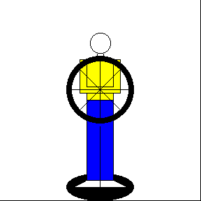
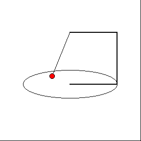
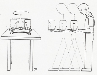
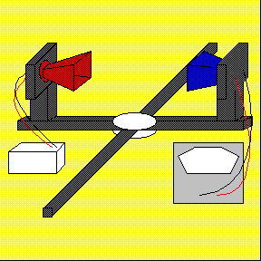
a. Have a volunteer stand on the turntable holding the bicycle wheel vertically. Start the wheel spinning and have the volunteer tilt it up or down towards a horizontal position. The demonstrator can steer himself around to any position with proper tilts of the wheel.
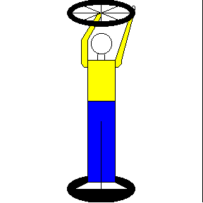
b. Stand on the turntable holding the bicycle wheel horizontally, and start it spinning yourself. You will start spinning the opposite direction to conserve angular momentum.
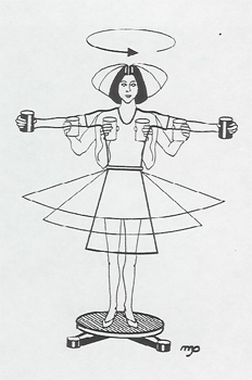
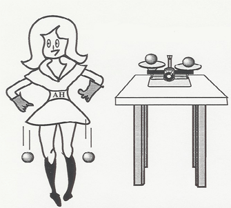
For the ice skater effect, have a student stand on the turntable with arms outstretched holding one or two kilogram weights. Start her spinning slowly, and then have her pull her arms into her chest. You must start her spinning quite slowly, or when she pulls her arms in, she will be thrown off the turntable.

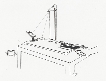
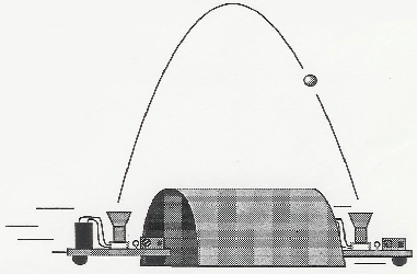
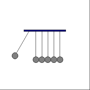
A spring gun, clamped to the lecture table, fires a steel ball into a pendulum bob, which traps it. The pendulum bob swings away and is held at the highest position reached by a ratchet. The laws of conservation of energy and momentum for the inelastic collision of the steel ball with the pendulum bob are used to calculate the velocity of the ball as fired by the gun from the data of the height of rise of the bob and the mass of the ball and the bob.
The pendulum bob is then moved out of the way so the gun can fire across the lecture hall. Tne laws of ballistics are used to calculate the spot on the floor the ball will hit, and a metal can is placed on the predicted spot to catch the ball.

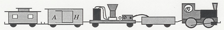
A toy LGB train has a flat car with a vertically mounted gun, actuated by a flashlight. When the train is at rest, the projectile ball is shot vertically upward and falls back down into the gun muzzle. If the train is moving along a straight section of track, the ball is still caught by the gun, even though the trajectory of the ball is now a parabola. The train can even be sent through a tunnel so the ball is fired up before the flat car enters the tunnel, passes over the tunnel, and is caught as the flat car exists the tunnel.
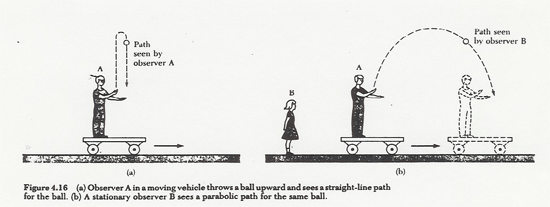
If the gun is fired as the train is rounding a curved section of track, the ball will not be caught, illustrating the restriction of special relativity to inertial frames.
This is a fairly elaborate demonstration, and several people are required to set it up, the set-up time often running five minutes or so into the beginning of class. Please give extra notice for your planned use.
![]()
Instructions
Do not run above 18 V. Train will wreck!
(There is probably a 2 V margin up to 20 V, but a wreck causes serious damage.)
The switch on the battery car turns on the system. Switch off after use to conserve batteries. (The switch on the gun car should be left on.)
llustrates that the vertically downward acceleration is independent of the horizontal velocity. See: Horizontal and Vertical Ball Drop (Gravitational Acceleration) [10].

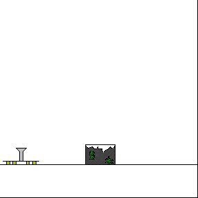
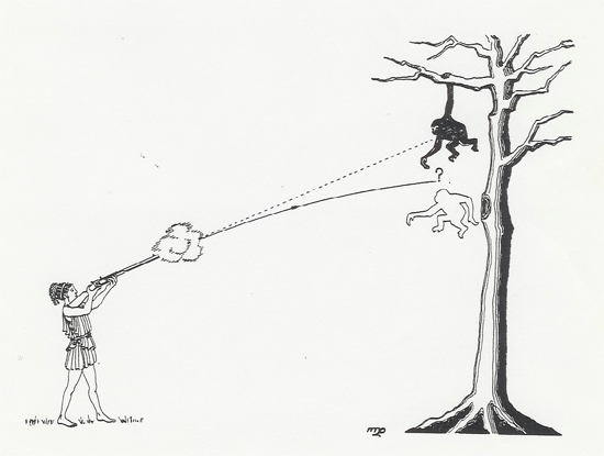
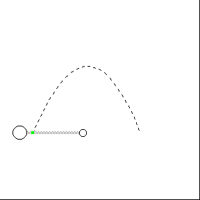
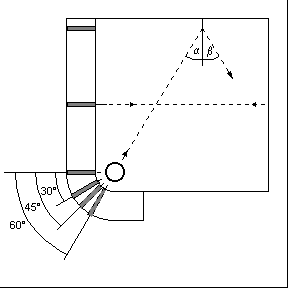
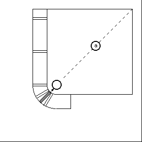
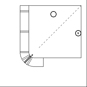
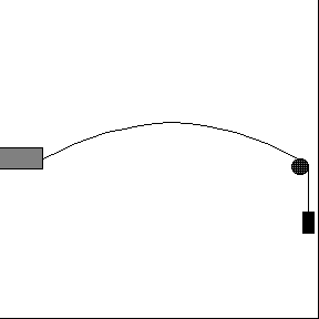
A monkey hanging from the branch of a tree in Africa is spotted by a small game hunter. But this is no ordinary monkey; this monkey knows some physics. He sees that the barrel of the gun is pointed directly at him and reasons that if he lets go of the branch at the right instant, the bullet will pass over his head. But he knows that the sound from the gun will not reach him much before the bullet, and maybe even after, so he decides to watch for the light flash from the gun, knowing that the light reaches him almost instantly, and to let go the instant he sees the flash. Is his reasoning correct?
Modern technology gives us a 25mm, laser guided, anti simian cannon. The monkey and hunter demonstration is on a wheeled table with the elevation of the gun controlled by a crank. The gun is fired by compressed air from a pressure cooker tank. A laser beams through the gun barrel so all can see where the straight line of the gun-aim is directed.
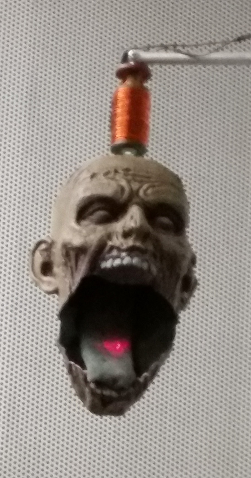
Besides a monkey target, we also have a zombie target, so if monkey hunter is not politically correct, you can call this, shoot the zombie instead. You can see a video test firing with the zombie here [11]. A picture of the zombie with the laser spot is shown below.
The illustration below is available on a viewgraph for overhead projection to the class.
Zombie head with laser spot.
Mouse over the animation below to see how the monkey hunter works at two different pressures.![]()
A ping-pong ball is placed inside the PVC tube and both ends are sealed with pieces of Mylar after which the tube is evacuated to ~ 10 Torr. When the Mylar piece near the ball end is punctured, the ball accelerates due to the expanding air behind it, leaving the tube at speed close to 300 m/s.
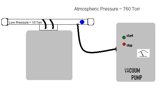
The ping pong ball can tear through two aluminum cans.
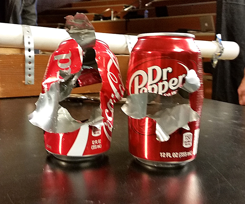
It is interesting to note that the Mylar piece used as a barrier at the exit end becomes detached before the ball reaches it. The following photograph is taken from G. Olson, R. Peterson, B. Pulford, M. Seaberg, K. Stein, R. Weber, The Role of Shock Waves in Expansion Tube Accelerators, Am. J. Phys, 74 (12), December 2006, p. 1071-1076.
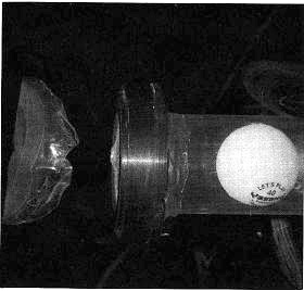
The explanation requires consideration of nonlinear gas dynamics and shock behavior. Compression waves traveling ahead of the ball quickly develop into a shock wave that reflects off the exit end of the tube and in turn off the ball several times. With each reflection there is a localized pressure and temperature increase so that by the third or fourth one a heated pressure pulse builds up at the exit end and is enough to remove the barrier piece.
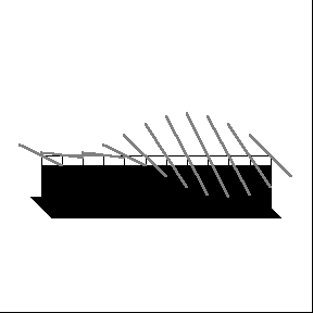
A spring gun is arranged to fire at various angles to illustrate that the maximum range of a gun occurs at 45°, the gun has equal ranges of the angles 45° �, etc.
Ballistic Motion is studied with a water stream that continually shows the parabolic trajectory of particles in a gravitational field. Measuring rulers hang down near the stream so that you can show, for example, that the stream falls a distance 1/2 gt� below the straight line it would have followed had there been no gravity. You can vary the angle of projection to show the 45° angle of greatest range, equal ranges at equal angles about 45°, etc. This demostration has audience appeal as the water pressure varies, and the instructor struggles to make the measurements while occasionally getting spritzed.
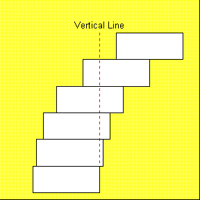
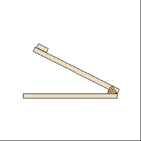
a. An irregularly sharped wooden block is suspended from various points, and a plumb line is dropped to determine the center of gravity.
b. A double cone will roll up an incline. (Actually the axis or c.m. of the cone descends because of the divergence of the rails.)
c. The leaning tower is unstable with the top in place, but stable when the top is removed.
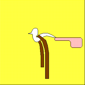
d. Hold your belt up with an otherwise unstable plastic bird.
e. A dumbbell with unequal masses on the end of a rod is suspended by s string to locate the center of mass. The dumbbell can then be tossed across the lecture hall to show that the center of mass follows a parabola, even though the ends are flying around. The center of mass is marked with phosphorescent paint which can be activated by ultraviolet light. Then in total darkness the students can see the dimly marked center of mass flying across the room in a parabola.
This oloid is composed of two circular disks which roll in such a way that the center of gravity stays constant.
If a series of identical rectangular blocks is stacked out at their balancing points from the top down, the top block can stick out arbitrarily far. You can show with a simple center of mass calculation the total "stick-out" distance; that is, the horizontal distance from the back of the bottom block to the back of the top block is 1/2(1 + 1/2 + 1/3 + 1/4 + ...). This series grows without limit.
Many students are surprised to see the top block "sticking out in space", no part of it over the bottom block of the stack. The series above shows that this can happen with a stack of only 6 blocks. In practice at least 6 are needed, and several more to make to effect dramatic.
This graphic demonstration of stability comes from Russia. When the line of the plumb bob hanging below the center of mass falls within the base, the prism is stable. But when the extended plumb bob line falls outside the base, the prism tips over. This demonstration is similar to the Tower of Pisa [12], and the two can be used together.
"Glasnost gives us this pretty demonstration from Russia. In Russia all students are required to take 5 years of physics, and these demonstrations are used throughout Russia. However, the Russians lost the Cold War so, though it pains me to say it, perhaps it is better to watch MTV than to study physics too hard!"
A beautiful wine rack demonstrates how, for stability, the center of mass must be over the support base.
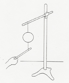
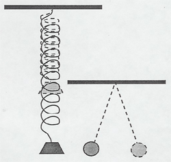
In this dramatic demonstration a massive weight is suspended by a wire from the ceiling of the lecture hall. The demonstrator stands braced against the wall, draws the mass to his nose, and releases it. If conservation of the energy holds, on the return swing the mass will stop just millimeters in front of his nose. But if conservation of energy fails,...!
The lengths of the pendulums in the corresponding lecture halls are as follows:
| PAB 1425 | 4.66 m |
| KNSY PV 1220B | 4.67 m |
 |
 |
A simple pendulum set swinging will rise to the same height on each side. If a bar interrupts its swing on one side, it will still reach the same height. The position of the bar is variable.
The ball rolling on the track will rise to the same height regardless of how the angle of the raisable side is changed

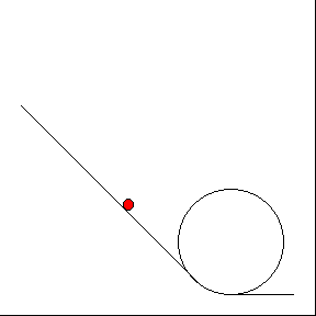
A ball is rolled down an inclined track which has a vertical 360° loop at the bottom. The rolling ball stays on the track if started from the proper height on the incline. Friction and the rotational energy of rolling must be taken into account. Note that the ball does not roll on its bottom, so it uses even more rotational energy than a rolling sphere.
 |
 |
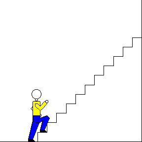
The maximum horsepower developed by a human being over a few seconds time can be measured by timing a volunteer running up the stairs in the lecture hall. If a person of weight W runs up height h in time t, then h.p. = Wh/t X 1/550 ft-lbs/sec. A person in good shape can develop one to two horsepower. It will be entertaining to the students if the professor tries it too.
Should the person be allowed a running start?
A small top, once set spinning, spins indefinitely. Can we reason that there must be some hidden, external source of energy to overcome the frictional loss of the top?

![]()
Many principles of mechanics can be nicely demonstrated with the Blackboard Mechanics Set. Among them are:
| Friction blocks on inclined planes | |
| Statics of inclined planes | |
| Levers and center of mass | |
| Vector addition of forces | |
| Pulley systems | |
| Pendula and springs |
A description book of various experiments is available.
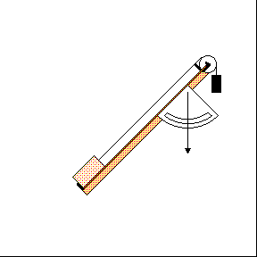
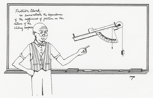
The effects of static and sliding friction are demonstrated on an inclined plane. The angle of the plane can be adjusted until the block just begins to slide. Or, a pulley, string, and weight can be used to pull the block up the plane at constant speed.
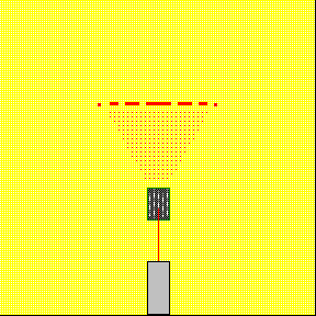
Terminal velocity is shown by dropping a ping-pong ball (with denser balls, if desired) from a platform and illuminating its fall with a strobe light. (See Three Balls Falling [7])
Please refer to: Acceleration Down an Inclined Plane (Kinematics) [13].
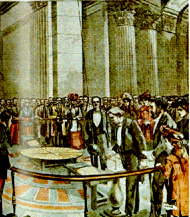
The universal gravitational constant G can be measured in class with the Cavendish balance; however, the demonstration is time consuming and delicate. A video tape of the demonstration has been prepared by Prof. C. Buchanan and Jim Abbott using time lapse photography of the optical lever readout. The tape is about seven minutes in duration and presents the students with the data of the experiment so the value of G can be calculated.
Drop a wooden ball simultaneously with a much heavier steel ball to show that they fall together. To show that the steel ball is definitely heavier, place the wooden ball in a short cup on one side of a double pan balance, and then put the steel ball in a short cup on the other side so the balance clunks down.
You might think that by this time everyone knows that a heavy object falls no faster than a light one - at least, everyone who had a high school physics course! But try asking in your Physics 10 class, "Will the heavy ball fall faster than the light ball, or the same?" You will be surprised at the variety of answers and justifications.
Then ask them about the effect of air resistance (which will probably already have come up in the discussion). To illustrate air resistance, take two sheets of paper, crumple one up into a ball, and drop them together. They have the same weight, but the flat sheet has more area "fronting the wind".
Lester Hirsch suggests a drama for jazzing up this last demonstration. Borrow the two sheets of paper from two different students. Tell them not to tear the pages out of their notebooks; you are going to return the pages. After the demonstration hand the flat sheet back to the first student, and carefully smooth out the crumpled sheet and hand it back to the second student. When he makes a face, tell the class that conversation has to start somewhere, and that he has to be one this time!
To make this demonstration somewhat more quantitative, you may wish project a slide of a wooden ball, a steel ball, and a ping-pong ball falling, photographed at 1/20 sec. intervals. (See Three Balls Falling [7])
As a final first-day demonstration, drop the "happy" and "unhappy" balls to show that objects that look identical may have very different physical properties.
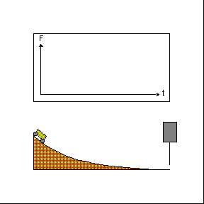
This demonstration shows that the top end of an upright rod, anchored at its bottom end, falls more rapidly than free fall. Several articles in the journals show how this effect causes a falling chimney to break about one third of the way from its bottom as it falls.
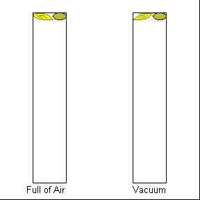
A coin and feather (or rubber cork and styrofoam chip) are inside a lucite tube 1.5 m long. When the tube is switched end for end, the rate of falling of the two objects can be compared. The tube is then evacuated to show that they fall at the same rate in a vacuum.
This experiment was repeated on the moon by Apollo 15 astronauts using a feather and a hammer. You can see the NASA video here [14]. We also have this clip on video disk which can be played in class.
A ball dropped vertically and a ball projected horizontally at the same instant hit the floor at the same instant.
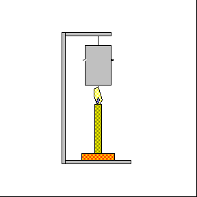
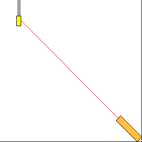
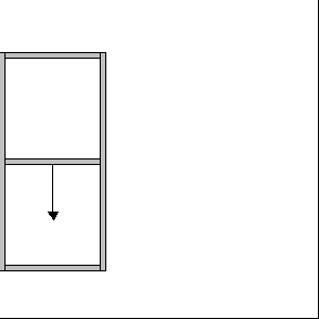
A coordinate frame in free fall in a gravitational field is truly inertial; that is, Newton's lst law is obeyed. In this demonstration a coordinate frame similar to that shown in the figure is held by an electromagnet. If the guns are fired while the frame is held, the projectiles will follow parabolic trajectories in the earth's frame and bounce off the intermediate plexiglass sheet. But if the frame is dropped, the guns firing automatically during the falling motion, the projectiles will follow straight lines in the falling frame and reach their target pockets.
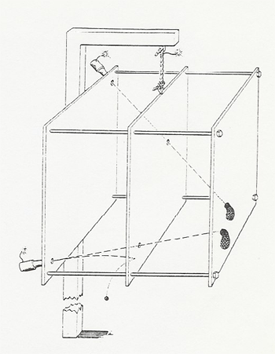
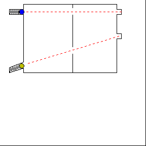
Note that this demonstration is equivalent to the Monkey and Hunter [3] demonstration.
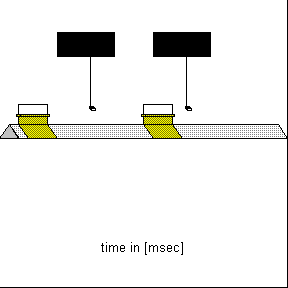
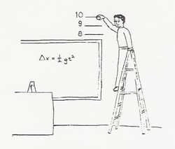
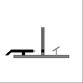
Simple Measurement of g: Heights of 6, 9, and 12 feet are marked up on lecture hall wall. Time intervals are announced by a metronome set to 80 beats/min. (Dt = 0.75 sec.) The demonstrator stands on a ladder and drops a ball from various heights on the beat of the metronome. Nine feet will be found to be the height for which the next beat is simultaneous with the ball hitting the floor. Then, g = 2h (Dt)2. This demonstration requires moderately good reaction time. A student volunteer may help. AVAILABLE ONLY IN KNUDSEN 1200

Measuring g with Sonic Basketball: In this experiment the kinematics of a basketball under the influence of gravity is studied quantitatively. The ball is thrown upward above a motion sensor to plot its position, velocity and acceleration as a function of time. (See Sonic Basketball [15])
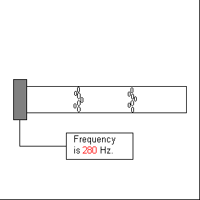
Three balls (steel, wood, and ping-pong) are suspended from a platform. As they are released, they are illuminated with a repeating strobe of known frequency. The result can be video taped with Video Point Capture. This software can be used to make measurements and analyze the motion of each ball as a function of time. A sample is shown to the right.
Two simple demonstration of weightlessness with minimal equipment are described below. (The Local Inertial Frame [16] is also a demonstration of weightlessness and the fact that Newton's First Law is obeyed in a freely falling frame.)
![]()
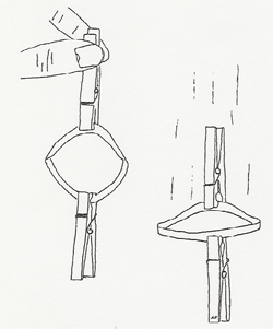
Clip two clothespins on the sides of a rubber band. Hold one clothespin and let the other hang down by the rubber band. The weighing of the second clothespin is represented by the stretching of the rubber band. Now release the upper clothespin. The rubber band goes slack, and the two clothespins and the rubber band fall together. The clothespin(s) are weightless when falling.
Suggested by Mr. Wizard.
![]()
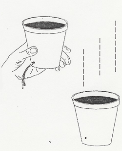
1. Punch a small hole in the side of a styrofoam cup or a 2 liter bottle near its bottom.
2. Hold your thumb over the hole as you fill the cup with water. Ask the students what will happen if you remove your thumb.
3. Remove your thumb and let the water stream out into a catch basin (a pail) on the floor.
4. Again seal the hole with your thumb and refill the cup. Ask the students if the water will stream out if you drop the cup as you remove your thumb.
5. Holding the cup as high as possible, drop the filled cup into the catch basin. The water does not stream out; the cup and water are weightless.
Suggested by Dale Bremmer.
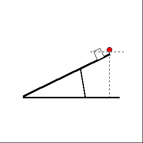
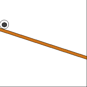
| A four meter long track is available for Galileo's "diluted gravity". Galileo argued that as the angle of incline of a track is increased, the motion of a rolling ball approaches free fall, so that the motion of the ball down the track is the same type of accelerated motion as free fall.
This device is very useful when you are discussing uniformly accelerated motion and free fall because motion is slow enough on the track so you can describe it while it is happening. For example, you can simulate a ball thrown in the air by rolling a ball up the track while discussing how its velocity decreases on the upward leg, becomes zero at the top, and increases on the downward leg. |
|
The concept of acceleration can be demonstrated by rolling a ball down the inclined plane and marking its successive positions on drafting tape pasted to the track, timing the positions with metronome beats. The simplest way to do this is to have several positions marked before the class begins and add a few more during the class demonstration, while showing the students that the ball passes all the marks at the right times. Then by measuring the distances you can show that the total distance the ball rolls increases with the square of the time.
Galileo's experiment itself is likely to be obscure to the students, since it depends on knowing that the difference of successive square integers are the odd integers. It can be performed as follows: The tape pasted to the track is marked as before, or perhaps by a student volunteer with good reaction time and coordination. The tape is then cut at the marks and pasted onto the blackboard in the form of a bar graph. The ratios of the heights 1 : 3 : 5 : 7 : 9 ... give the differences of the squares in the formula y = 1/2 at2.
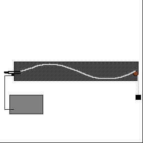
A sonic ranger measures the distance to a moving object by bouncing ultrasonic sound off the object and timing the echoes. The data, taken about every 0.05 sec. is read into a computer which then plots the distance, velocity, and acceleration. The results can appear on overhead projection via the LCD screen, or in some rooms, directly on video projection. Derivatives, integrals and other manipulations of these quantities can be performed. Three typical experiments are described:
|
|
1. A cart is sent up a tilted Pasco track to roll back down. This is a good demonstration to illustrate kinematics concepts since the students can see distance, velocity, and acceleration plotted simultaneously. |
| 2. A plate is supplied which the instructor can move in various ways to again illustrate d, v, and a. Start simple; hold the plate at constant position for a few moments, move at constant velocity to a new position, and hold this new position for a few moments. Have the students predict the graphs of d,v, and a. |
|
 |
3. A pendulum is set swinging and the computer plots out the sine and cosine waves of d, v, and a. Their phase relations can be pointed out. Try reassigning the axes to plot d against v. |
Several different sonic rangers with their associated software, computers, and projection equipment are presently being tried in the classrooms. Plan on familiarizing yourself a little with the specific equipment before using it in your class.
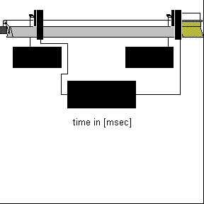
Data Studio [17] is used with Pasco probes to demonstrate the kinematics of one-dimensional motion.
Measurements of Position, Velocity and Acceleration of Constant Linear Motion
Equipment: Computer, 2.2m Pasco track, Cart, Motion Sensor and Metal Slugs.
The above equipment is used in conjunction with Data Studio to measure and plot the position, velocity and acceleration of a Pasco cart as a function of time. During lecture the instructor can show quantitatively that at each instant the velocity and acceleration are the slopes of the line tangent to the position vs. time and the velocity vs. time curves respectively. Data Studio can also be used to obtain the average velocity and acceleration of the cart.
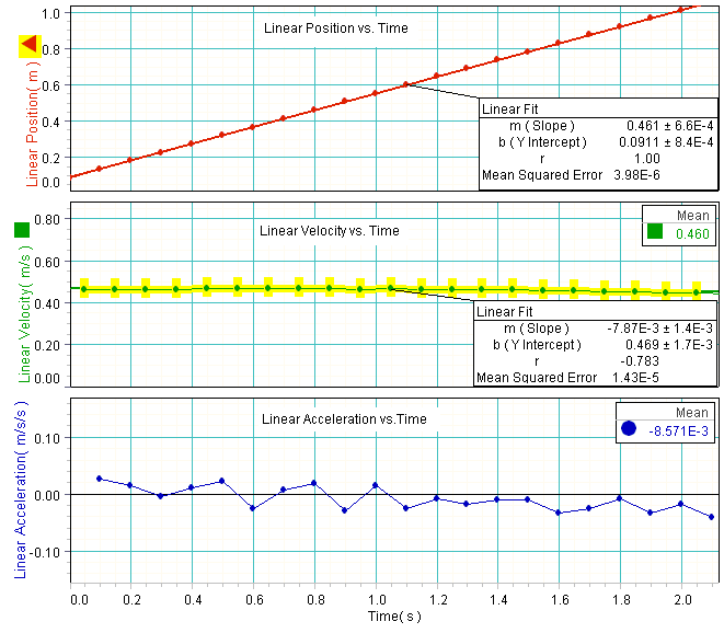
In the following Data Studio experiment, the Pasco track was propped up slightly on one end with adequate metal slugs to compensate for friction. Then the cart was given a slight push to achieve constant velocity. The motion sensor was used to measure and graph the cart's position as a function of time. The graph shows that the position changes linearly as a function of time. A linear fit to the position vs. time curve gives the slope to be 0.45 m/s. This constant value corresponds to the average and instantaneous velocities for this experiment. Furthermore, it is within experimental error of the mean of the velocity vs. time curve (0.46 m/s). Taking the slope of the velocity vs. time curve, we find that it is zero and therefore have zero acceleration -- also demonstrated experimentally.

Measurements of Position, Velocity and Acceleration of Nonlinear Motion
The acceleration graph is made by taking the tangential slope of the velocity vs. time curve at each point and plotting this value as a function of time. Data Studio is then used to calculate the mean of the acceleration vs. time curve where we find the value to be -9.2 m/s/s. The values obtained by the linear fit to the velocity vs. time fit from above and the mean of the selected data points of the acceleration vs. time graph are in general agreement and close to the accepted value of gravity of 9.8 m/s/s.
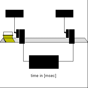
Instantaneous Velocity, Average Velocity, and Acceleration using the Air Track
Below is a sample set of demonstrations with an air track for illustrating these concepts using a clock (the "white clock") that measures the elapsed time for a glider to travel one meter and another clock (the "red clock") that measures the time for the 0.1m flag of the glider to pass a sensor at the end of the one meter interval.
1. First explain exactly what the clocks are measuring to the students. A transparency is available that can be projected during the demonstrations to remind them what is measuring what. Show them that the white clock measures the elapsed time for the glider to travel one meter by passing your hand through the start-gate, counting off "one thousand one, one thousand two, " for several seconds, and then passing your hand through the stop-gate. Then show them that the red clock measures the time for the glider flag to pass its sensor by blocking its gate with the glider flag, counting off several seconds, and removing the glider.
Then if the white clock reading is labeled T and the red clock reading is labeled t:
average velocity = 1 meter/T
instantaneous velocity = 0.1 meter/t
At some point you may wish to discuss how the exact instantaneous velocity is defined in terms of the calculus derivative by imagining the flag length to become smaller and smaller.
2. To check that everyone understands what the clocks are measuring, ask them, "If the track is level and I send a glider through the gates, what will be the relationship between the readings of the two clocks?" (And then do the demo!) Answer: red clock reading = 1/10 white clock reading.
3. Now use a block to tilt the track up. Ask, "The red clock should now read (greater than, less than, the same as) 1/10 the white clock. In other words, is the instantaneous velocity at the end of one meter of acceleration (greater, less, the same) as the average velocity over the one meter distance?"

4. Now use a larger mass glider. "The clock readings should be (greater, less, the same as) before?"
5. "At what fraction of the one meter distance does the glider attain an instantaneous velocity equal to the average velocity over the one meter? In other words, where should the red sensor be placed to get red = 1/10 white with the track tilted?" (Answer: 1/4 meter)
6. You can check the measured acceleration against the tilt of the track. If the track length is L and it is tilted height h,
acceleration = a = g sin q = gh/L
Then from the white clock, a = 2 meters/t2 a = 2 meters/T 2
and from the red clock, a = (0.1m/t)2/2m = 0.005 meters/t2
Data Studio [17] is used with Pasco probes to demonstrate the kinematics of one-dimensional motion under gravity.
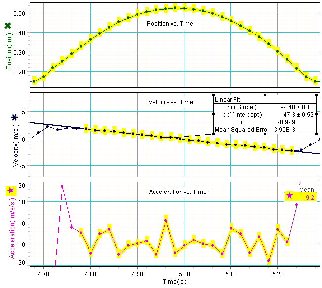
Equipment: Computer with Data Studio software, Sonic motion sensor and basketball
In this experiment the kinematics of a basketball under the influence of gravity is studied quantitatively. The ball is thrown upward above a motion sensor to plot its position, velocity and acceleration as a function of time. The graph below shows that the ball's vertical position changes quadratically as a function of time while its vertical velocity changes linearly. The tangential slope of the position curve is taken at each point to calculate the velocity vs. time plot. The ball's velocity is a maximum as the ball is first thrown upward, zero at the ball's maximum height, and negative its maximum value when the ball returns to its initial starting position. By using Data Studio's fitting algorithm, a fit to the velocity vs. time curve is found and the slope is calculated to be -9.48 m/s/s as shown.
The acceleration graph is similarly computed by taking the tangential slope of the velocity vs. time curve at each point and plotted as a function of time. The mean of the acceleration vs. time curve is calculated by Data Studio to be -9.2 m/s/s. The numbers obtained by a linear fit to the velocity vs. time plot from above and the mean of the selected data points of the acceleration vs. time graph are in general agreement and close to the accepted value of gravity of 9.8 m/s/s.
Measure the velocity of a speeding bullet using a totally inelastic collision. (See Ballistic Pendulum (Ballistics) [18])

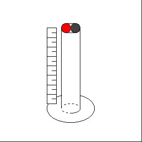
Various balls are dropped in a transparent tube to show nearly elastic, partially inelastic, and totally inelastic collisions. The height of the bounce, marked off qualitatively on the tube, is a measure of the elasticity. A lead ball which does not bounce at all is startling.
With another piece of apparatus a small steel ball is dropped on a heavy, polished, slightly concave steel plate. The collisions are so elastic that the ball bounces dozens of times before its energy is exhausted.

With the collision ball apparatus one can show that if a moving ball collides elastically with an equal mass ball at rest, the entire kinetic energy and momentum of the first ball will be transferred to the second.
If one ball collides with a row of equal mass balls, all the kinetic energy and momentum will be transferred to the last ball.
One larger mass ball is provided to show the dependence of these results on the mass of the colliding ball.
An interesting experiment is to pull back two balls on one side and one on the other and release them simultaneously.
|
|
A. Understanding car crashes - It's Basic Physics, put out by the Insurance Institute for Highway Safefy and narrated by a high school physics teacher. This video is a more modern version of the Crash Test Dummies video to illustrate Newton's second law in the context of car collisions. The video uses scenes in which an egg is thrown at a brick wall and sheet to demonstrate momentum transfer and impulse. The typical running time of the appropriate segment of video is less than five minutes and the entire video is twenty-two minutes.
B. "Physics and Automobile Collisions" by Dean Zollman - This laser disc video illustrates the concepts of Newton's Laws, impulse and momentum, conversion of kinetic energy to other forms, and conservation of momentum in 2D collisions with physics narration. You may wish to watch the disk through and pick out parts appropriate for your class, or I recommend the following parts as a short general survey:
| Chapter 1 | Introduction | 38 sec |
| Chapter 2 | 1st Law, impulse and air bags | 2-1/2 min |
| Chapter 4 | Price of damage to car with and without shock absorbing bumpers | 1-1/2 min |
Elastic and inelastic collisions between carts can be demonstrated as one end of the carts are equipped with magnets and the other end with Velcro. A moving cart collides elastically with a stationary cart of equal mass using the magnetic ends. The originally stationary cart moves away with all the velocity. Elastic collisions between carts of different masses can be tried qualitatively or quantitatively with Data Studio.
Completely inelastic collisions result by colliding the Velcro ends of the carts. A carts velocity is measured before and after it has collided inelastically with another cart of equal mass. It is demonstrated that the velocity of the two carts after the collision is half the initial value.
|
Elastic Collision |
Inelastic Collision |
|---|---|
|
|
|
Explosions are demonstrated by touching the ends of two carts together and releasing an internal plunger from one of the carts.
|
Explosion |
|---|
|
|
All of the above demos may also be demonstrated with the air track at the instructor's request. The air track has an advantage over the dynamics track in that there is less friction associated with it. However, the air track has a draw-back in that it is much nosier than the dynamics track and in a lecture setting it is difficult for the instructor to be heard.
Two identical looking balls are suspended as pendula. One at a time they are lifted up to swing against a standing block. One ball easily knocks the standing block over, but the other does not. There is another pair of balls so you can show that the "happy" ball is elastic and bounces high, whereas the "unhappy" ball is totally inelastic and does not bounce. (F. Bucheit, Physics Teacher 23, 28, 1994).
Two battery-operated air cushion disks are available for demonstrating two-dimensional elastic collisions. Simply collide one disk into the other on the floor of the lecture hall.
Law of Reflection
Elastic Collision Experiments
This demonstration displays the impulsive force in a collision as a function of time using the Pasco dynamics track. The track is elevated at one end and the cart is allowed to accelerate with the force sensor connected. Data Studio [17] is used to measure and plot the force as a function of time. The momentum is just the area under this curve.
Choose two students, one heavy and one light, and stand them on the large reaction carts. When they push on each other's hands, the light student acquires a proportionally larger velocity than the heavier student.
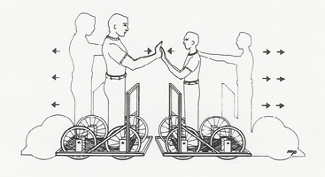
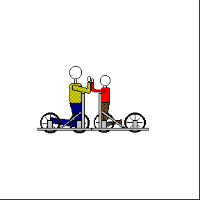
Small reaction carts illustrate the same principle on the lecture table, as do gliders on an air track connected by a compressed spring.
Ask your students to answer from:
A. heavier person
B. lighter person
C. both the same
Which person feels the greater force? Which person gets the greatest impulse? Which person undergoes the greater change in momentum? Which person undergoes the largest acceleration?
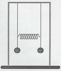
This pretty demonstration illustrates two principles: one, the period of a conical pendulum is the same as a linear pendulum; and two, all the momentum is transferred in an equal mass elastic collision.
Two identical ivory balls hang side by side from the ceiling of the lecture hall. You can illustrate the equal mass collision by pulling one out and letting it collide with the other, as in the Collision Balls [19] demonstration. Now pull both balls back, away from the class, hold one lightly with your fingers, and collide the other into it from the side. The colliding ball will stop "dead" and swing toward the class in linear pendulum motion, and the struck ball will swing around in conical pendulum motion. Since the periods of the motions are the same, the balls will again collide at the end of the swing and exchange motions. The situation will continue for some time with the balls exchanging conical and linear pendulum motion at successive collisions.
Available only in the Knudsen Lecture Halls and PAB 1425
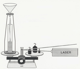
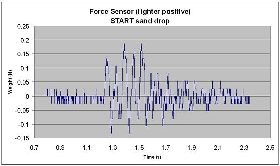
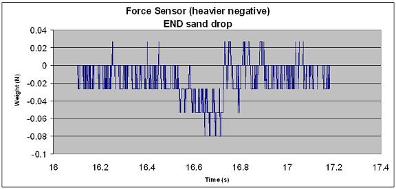
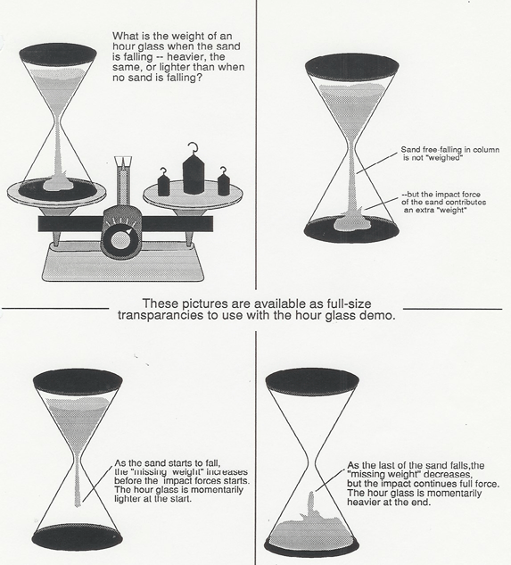
Does the weight of an hourglass change when the sand is falling? This demo shows the truth! A funnel with the sand held back by a cork and string arrangement is perched to drop sand into a glass beaker on a double pan balance. A laser bounces a beam off a small mirror attached to the pointer of the balance. When you burn the string, the sand starts falling, and the motion of the laser spot on the blackboard indicates the result. A set of transparencies to use with this demo is shown below.
| The sand in the falling column does not contribute to the weight reading. But you can easily show from Newton's Second Law in the form F = dp/dt that the extra impact force of the falling sand exactly equals the missing weight of the total falling column of sand. Thus, while the sand is falling and impacting, the weight of the hourglass is equal to its weight when no sand is falling.
But initially, as the sand starts falling, there is "missing weight" in the column before the sand hits bottom, so the hourglass grows momentarily lighter. Similarly, at the end there a few moments while the impact force remains constant as the falling column decreases to zero, so the hourglass grows momentarily heavier. The movements of the laser spot on the blackboard faithfully trace out the graph of the weight of the hourglass as a function of time. |
|
| A movie clip of the typical setup is shown on the right. Note the position of the laser spot as the sand begins to drop and as its level in the funnel changes. The graphs below were produced with data from a setup using a PASCO force sensor in place of the scale. |
 |
 |
The Paul Trap, or rotating saddle trap, is an analogy to RF-electric quadrupole ion traping.
The Loop the Loop track can be reintroduced here, and the rotational energy of the rolling ball added to the calculation of the height that the ball must be released to just make it around the track. Note that the ball does not ride on its bottom, but partly up on its sides. You will still need to add in "a couple of inches of friction." (See Loop the Loop (Energy) [20])
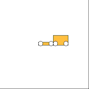
Various objects are raced down an inclined plane. There are two sets of disks, one with the mass distribution concealed and the other with the mass distribution apparent. All of the three inch disks have the same mass which you can demonstrate by placing two at a time on a double pan balance. There are also a few smaller disks available so you can demonstrate that disks of the same mass distribution but different sizes and masses roll the same.
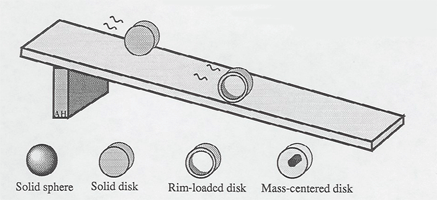
Unidentified Rolling Objects (Audience Appeal)
These demonstrations are often shown with the rolling objects above, or on the first day of class, or at physics demonstration shows, to attract interest in physics, and as an illustration scientific reasoning in working out their mechanism "How would you design a mechanical system to do this?"
One of the "unpredictable disks", shown above, rolls down and one rolls up. The off-center weight is concealed from the audience, but can be shown after they have tried to reason out the mechanism. A "prematurely-stopping cylinder" rolls part way down and stops. A "come-back disk" rolls down some distance, and then rolls back up!
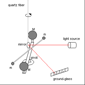
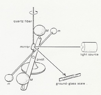
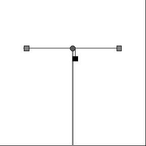
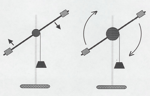
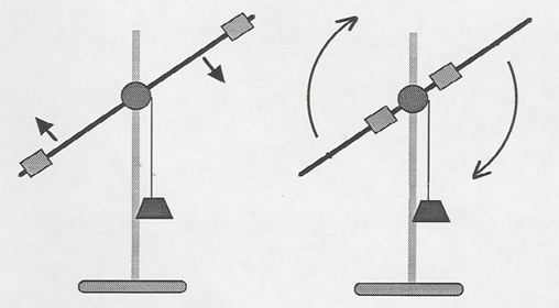
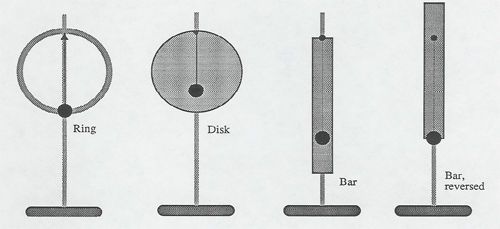
This simple device graphically illustrates the concepts of torque and rotational inertia. Movable masses are positioned on a rod which is rotationally accelerated by a falling weight. The rod arm accelerates rapidly when the masses are moved in toward the center but much more slowly when the masses are adjusted out to the ends of the rods so that the rotational inertia is large. Two devices are available so that the class can directly compare the cases of large and small rotational inertia.
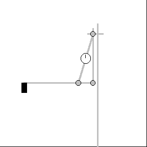
The Position of masses on rods can be varied to change the rotational inertia of a torsion pendulum. The period of the pendulum is longer for larger moments of inertia. The torque of the support wire accelerates the rotational motion more slowly when the rotational inertia is large. (See Simple Harmonic Motion [21])

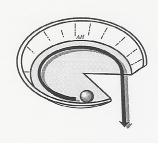
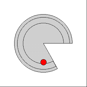
Illustrates how changing the rotational inertia changes the angular velocity. (See Turntable and Weights (Angular Momentum) [4])
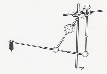
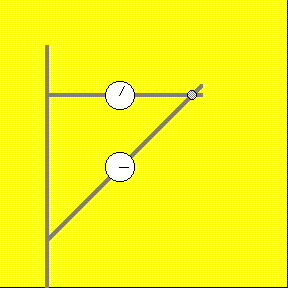
The model shown below, constructed from the strut and tie set, demonstrates the force a human biceps muscle must exert when a weight is lifted by the hand.
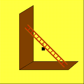
A wooden model of a ladder leaning against a wall demonstrates the angle that the ladder will slip down when weights are hung from various rungs of the ladder.
Statics of inclined planes, levers etc. can be done with the Blackboard Mechanics Set [22].
A multiple strut and brace framework can be set up on the lecture table. Force indicators (indicating newtons) are placed in the framework to show the balanced forces. The biceps muscle shown above is an example. An instruction manual showing various set-ups is available (hoisting, wall crane, roof truss, etc.).
Illustrates that the torque of gravity, acting on a stick hinged at its base to the table, causes the end of the stick to accelerate faster than g. (See Falling Chimney (Gravitational Acceleration) [23])
A bicycle wheel can be mounted on the lecture table so you can illustrate the effect on acceleration of exerting forces on it at various radii and in various directions. A crescent wrench is also supplied so you can illustrate how to produce the maximum torque on the nut holding the bicycle wheel. Another simple illustration of torque is to open the door to the lab at the front of the lecture hall and push on it at various radii from the hinge with your index finger. The crumpling of your finger indicates the larger forces needed at the smaller radii.

A more quantitative demonstration of torque uses the rotational acceleration device shown here [24]. The spindle is fitted with a spool of twice the radius of the shaft so the falling weight acts at 2R. Two devices are available. Adjust the weights so the rotational inertia is the same, and compare the rotational acceleration of the devices with the falling weight acting at R and 2R.

Add hanging weights at different distances to break the hold of the friction nut. It takes twice the weight at half the distance. Watch out for your foot.
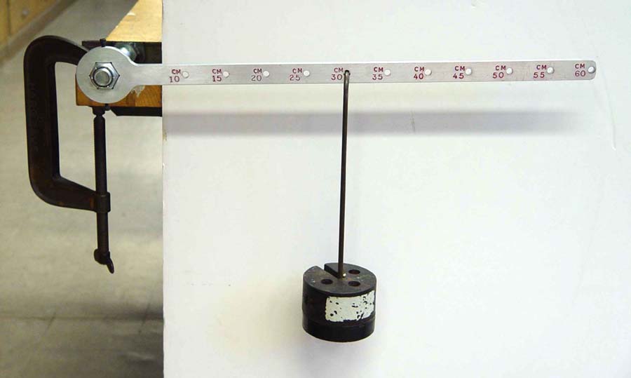
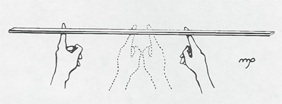
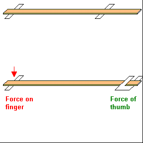
Hold a meter stick at two arbitrary places with your two index fingers. When you bring your index fingers together, they will meet at the center of the meter stick. You can show that this is a consequence of the two different friction forces resulting from the different torques exerted by your fingers. Amazingly, even if the coefficients of friction are very different, say by covering one finger with slippery chalk dust and the other with a sticky rubber glove, your fingers will still meet at the center. If a weight is placed on one end of the meter stick, the fingers will still meet at the balancing point, the center of mass.
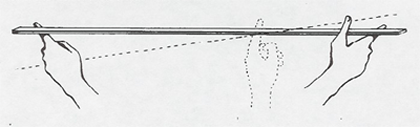
Professor Peter Schlein suggests this further demonstration of torque: Hold one end of the meter stick between your thumb and finger as shown above, and slide your index finger in from the other end. The force on your sliding finger increases from half the weight of the meter stick when your finger is at the far end to the full weight when your finger is at the center and the whole weight of the meter stick balances on one finger. As you slide your finger beyond the center towards the held end, your thumb must now exert a downward force, and the force on your sliding finger becomes extremely large. You can calculate the torques by assuming that the weight of the sections of the meter stick act at the centers of the sections.
The little ball lifts the big ball - a string connecting a large and small ball passes through a tube. When the tube is whirled around, the small ball moves out, lifting the large ball.
Get both balls out - a tube is arranged so that balls fall into pockets at its ends. It is impossible to get both balls into their pockets by tilting the tube around, but if the tube is rotated, both balls move into their pockets.
Various devices fit on the variable speed rotator below:
A mass extends a spring allowing measurement of the centripetal force.
Two balls move out on rods extending a spring to measure centripetal force.
Four balls move out on semicircular wires.
Spherical shape becomes oblate when rotated.
A spinning circular chain forced off a disc by means of a stick, retains its circular shape as it rolls rapidly along the floor.
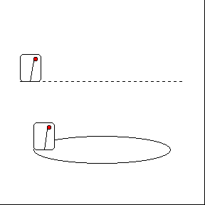
A strap of spring steel is pivoted from the center of a platform on a rotating turntable. The strap has a nail in its end so that as it falls from a standing position, it impales itself on the periphery of the platform. When the turntable is not rotating, the strap falls normally to a marked position. But when the turntable is rotating, as the strap falls the turntable continues to rotate, and the Coriolis "force" causes the strap to impale itself somewhat behind the previous mark.
In this simple demonstration a pendulum is mounted on, and suspended over, a rotating turntable. As the turntable rotates underneath, the pendulum maintains its plane of swing.
This device consists of a tethered ball floating in a jar of glycerin. To establish its operation, hold it in front of you, and begin rapidly walking across the lecture hall. The ball will move forward in the direction of your acceleration at first, and then return to the vertical position as your velocity becomes constant. When you stop walking, the ball will move back towards you showing a deceleration.
Now that you have demonstrated that the ball moves in the direction of acceleration, place the device on a turntable and start it rotating. The ball will move inward showing the radially inward uniform circular acceleration.
Put a liter or two of water into the bucket. Slosh a little out on the floor to show there is water in the bucket. Then swing it in a circle around your head.
"I like to have the students 'participate' in the demonstrations, so I'll walk up into the middle of the audience to swing the bucket around. See, it's not hard! No problem at all keeping the water in! Now let see how slow I can swing it and still keep the water in!"
Swing a tray with wine glass
For a more dramatic demonstration of uniform circular motion, fill wine glass half full of water and place it on a tray with three nylon ropes connected to it. Then swing the tray around. Stopping is a bit tricky so make sure to practice beforehand. This demo really holds the students' attention and excites them - especially if the glass breaks!
The simple set up shown below, suggested by Prof. P. Schlein, is a good illustration of the vector addition of forces. The vertical angle of the strings can be measured with a large protractor.
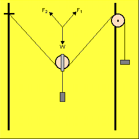
Various similar arrangements can be done with the Blackboard Mechanics Set [22].
This device operates on a view graph for the whole class to see easily. Angles are measured by the circular protractor; magnitudes of the forces by the extension of the springs via Hooke's Law.
Label the rings one through seven, starting with the first black ring beyond the last red ring. The force in grams weight as measured to the base of the cone forming the vector arrow is:
|
Ring |
Force |
| 1 | - |
| 2 | 50 gms |
| 3 | 85 |
| 4 | 120 |
| 5 | 155 |
| 6 | 190 |
| 7 | 225 |
Force in gms. wt. = 35 X ring # - 20
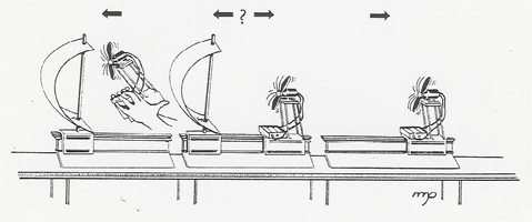
A good illustration and exercise in adding vectors is provided by a sailboat. The situations of "running with the wind", sailing crosswind, and sailing "close to the wind" are well reviewed in Epstein's Thinking Physics, 2nd Ed., pp 32 - 37. All of these examples can be demonstrated on the air track using a glider with sail and an electric fan to produce the wind. You can actually get the glider to move forward about 45 degrees into the wind.

Vector Addition
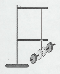
This apparatus consists of a platform that rolls along the lecture table, and some toy bulldozers or carts to roll on it. You can push the rolling platform with your hand or let a bulldozer push it. The angle between the motions is completely adjustable. The demonstration can be shown in several versions:
A. As a qualitative illustration, let the bulldozers move and sketch the resulting vectors on the blackboard.
 |
 |
B. To illustrate the path of a boat crossing a river, set the bulldozer rolling on the platform at slight back angle and mark a direction perpendicular to the platform motion on the lecture table with blocks. With the correct adjustments, the bulldozer moving on the platform will be seen to cross the shortest distance perpendicular to the "current".
C. The apparatus is set up on butcher paper, the initial positions of the bulldozers marked, and their final positions marked after the bulldozers have moved. Then the butcher paper can be taped up on the blackboard and the vectors sketched in.
D. In an elaborate demonstration, apparatus is set up as in the illustration above with a bulldozer pushing a blinky while a picture is taken of three blinky tracks as first one bulldozer moves, then the other, and then both. The picture is developed in ten seconds and projected on the screen so the students can see the three blinky tracks.
Magnetic arrows are available which can be stuck on the blackboard. Arrows come in various lengths and can be placed tip to tail to demonstrate vector addition. A protractor and ruler are also available to measure the angle and length of the resultant vector.
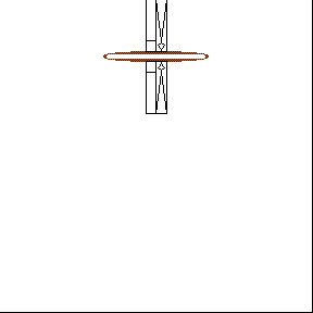
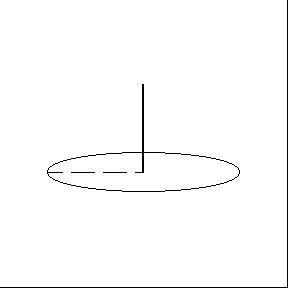
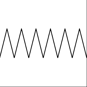
A simple demonstration of a radian. Is shows the relation between the radius and the section of circumference of a circle. A straight radius is lifted off and placed on the curve of the circumference. The angle bounded is one radian.
Data Studio is a data acquisition, display and analysis program. The software works with PASCO sensors and interfaces to collect and analyze data in real time. UCLA Physics and Astronomy Lecture Demonstrations has developed numerous experiments for use with undergraduate lectures to demonstrate physics concepts. Some of the concepts that can be shown include the following:
The relation between position, velocity and acceleration (p,v,a plots).
Conservation of momentum and energy.
Heat engines (PV and TS plots).
The relation between pressure and temperature at constant volume (PT at constant V plots).

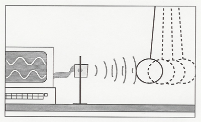
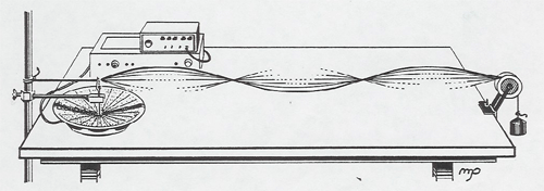
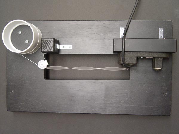
Two solenoid coils connected by wires are arranged so that magnets on springs oscillate in them. When one magnet is set oscillating, the induced current causes the other to oscillate also. Note that the oscillations are coupled through the velocity term rather than the amplitude term as in coupled pendula.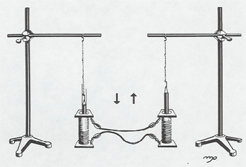
Also Current Coupled Coils (Electrodynamics) [26]
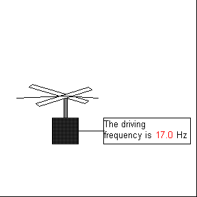
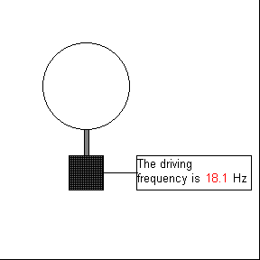
A Pasco apparatus gives digital readouts of the natural period of the oscillator, the driving frequency, and the amplitude of oscillation. A flashing LED shows the phase angle between driving force and the oscillator. This is the type of instrument that is even more interesting to the professor than the students. The driving frequency and amplitude, spring constant, mass, and damping can all be varied. You can quantitatively measure amplitude versus time (undriven), amplitude versus driving frequency, phase angle versus driving frequency, transient response, etc.
We also have a horizontal version with variable magnetic damping, using the Pasco track and a cart connected by a spring to a sinusoidal drive. This version has no electronic readout.
With this nice piece of apparatus you can vary the driving frequency and amplitude, and the damping (electromagnetic). Essentially the same concepts as above can be illustrated, minus the electronic readouts.
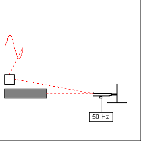
This demonstration is similar to Laser Sine Wave from Tuning Fork [27], but the tuning fork is now driven by a magnet coil connected to an audio oscillator. Normally the beam is not scanned with the rotating mirror, but one merely observes the amplitude of oscillation on the wall. One can demonstrate resonance by observing the large increase in amplitude when the oscillator is tuned to the natural frequency of the fork. If the oscillator is tuned slightly off resonance, beats between the driving frequency and the natural frequency are observed.
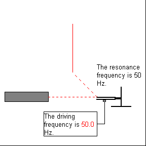
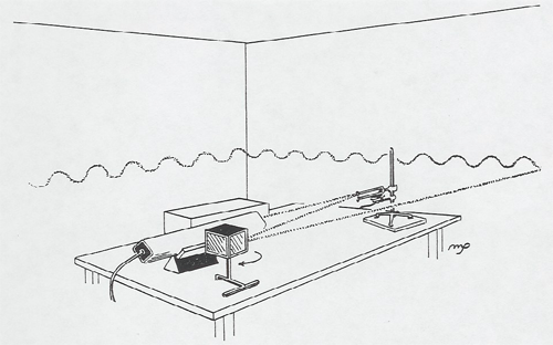
This impressive demonstration shows that the simple harmonic motion of a tuning fork is really a sine wave in time. A laser beam is bounced off a mirror on the end of a tuning fork to a rotating mirror which provides the time axis. The tuning fork is driven by an interrupted magnet.
- This information is from Bob Keolian.
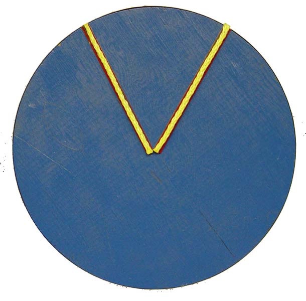
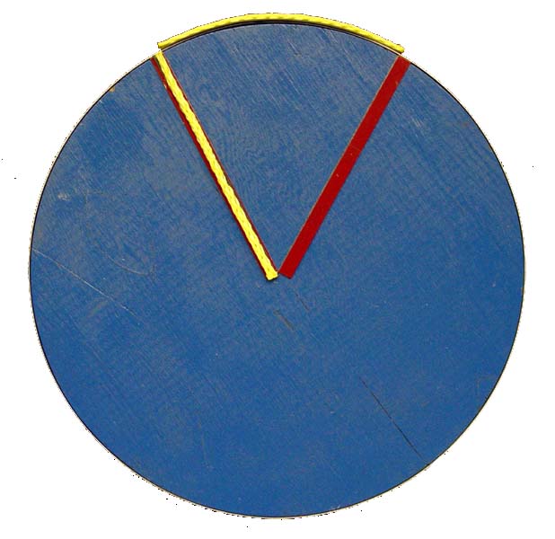
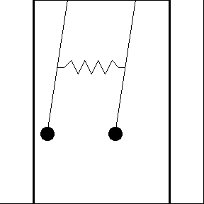
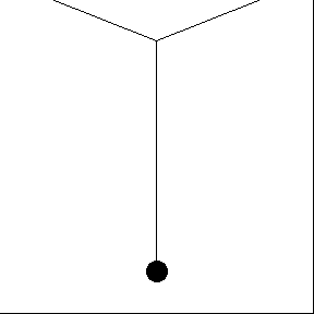
The trick is in the suspension. At the "Mystery Spot," a tourist trap in Santa Cruz, they suspend the pendulum with a chain by casually looping the chain around a horizontal beam associated with the roof of a shed. The chain reattaches to itself, forming a "V" at the top. Your's must do something similar, forming a V at the top, with two fixed attachments at the top of the V and a knot or some other junction at the bottom of the V to a single chain or rope that goes down to the pendulum. The trick is in noticing that for motion perpendicular to the plane of the V, the effective length of the pendulum is from the two attachments at top to near the center of mass of the pendulum below, but for motion in the plane of the V, the junction or knot point remains fixed and the effective length of the pendulum starts from there. This gives a shorter length and slightly higher frequency for motion in the plane of the V than for motion perpendicular to the plane of the V.
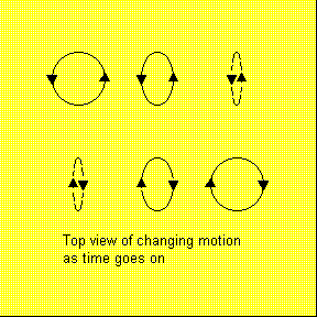
At reasonably small amplitudes, say less than about 10 degrees of deflection, the motion of the pendulum can be considered to be a linear superposition of in-plane and out-of-plane motion, with two modes of slightly different frequencies. So you can get different Lissajous figures depending on how you start off the pendulum. If you start off with a circular motion, you are exciting both modes with the same amplitude but with an initial 90 degree phase shift between them. As the modes progress in time, the instantaneous phase between them (w_1t - w_2t - initial phase) changes with time. Eventually, the two modes are in phase and the pendulum move in a straight line 45 degrees from the plane of the V. Later the phase is such that the circle changes direction. If you let the pendulum go, the pattern repeats itself. But that isn't as much fun as stopping the pendulum after it has reversed direction once and cooking up some BS story about a gravitational or magnetic anomaly in the mantle below Los Angeles that causes the change in direction.
If you start the pendulum off in planer motion either in the plane of the V or out of the plane of the V, then you excite only one of the modes, and the motion stays in its plane. At larger amplitudes the linear superposition of modes picture breaks down, at around 30 degrees of deflection. The two modes couple parametrically by modulating the tension in the rope at twice the oscillation frequency, but that is another story.
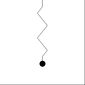
Parametric oscillation occurs when one of the parameters of the system is varied. A child can "pump" a swing by standing and raising and lowering her center of mass periodically, changing the length of the pendulum. The child pumps at twice the pendulum frequency, generating a sub harmonic.
A very simple demonstration of parametric oscillation is the coupling of the pendulum mode to a mass on a spring. When the spring frequency is approximately twice the swinging frequency (pendulum mode), the spring mode parametrically drives the pendulum mode, but the pendulum motion causes the tension in the spring to vary at twice the pendulum frequency, and therefore resonantly drives the spring mode. The transfer of energy between these two modes is impressive.
This exhibits wave like behavior, but the wave is an illusion. The pendulums are independent.
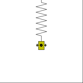
1. The Driven Mass on a Spring [28] can be easily set to resonance. Measure the natural period with the LED readout and then drive at the inverse, the natural frequency, also measured by the LED readout. Or adjust the phase between the driver and oscillator to 90 degrees lag as shown by the phase readout.
2. Resonance can also be found for the Driven Torsion Pendulum [29]. This is a little more difficult since there are no electronic readouts and the Q of the torsion wheel is quite large.
3. The Driven Tuning Fork [30] demonstrates resonance at high Q. as the frequency synthesizer is adjusted in steps of 0.1 Hz near its resonant frequency.
4. In Beats and Sympathetic Vibration [31], see show how one vibrating tuning fork can acoustically induce vibrations in another nearby, if it is tuned to the same frequency.
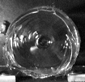
5. A dramatic demonstration of resonance in Breaking Glass with Sound [32].
Along with this we have the Tacoma Narrows Bridge collapse on video.
6. The Pasco track can be connected to a sinusoidal drive to demonstrate a driven simple hormonic oscillator. When the motor drive matches the resonance of the system, energy gets pumped in and the amplitude of the oscillations grow dramatically. This system can also be used to show a critically damped and under damped system by bringing an aluminum sheet close to two magnets attached to the cart.
7. A new demonstration is "resonance strips". Several metal strips of increasing length are bolted together in a star shape. When the device is vibrated with a mechanical driver controlled by a signal generator, the different strips come to resonance in the range 10 50 Hz by vibrating strongly at different frequencies according to their lengths. The class can see the frequency of the driver on a large display frequency counter.
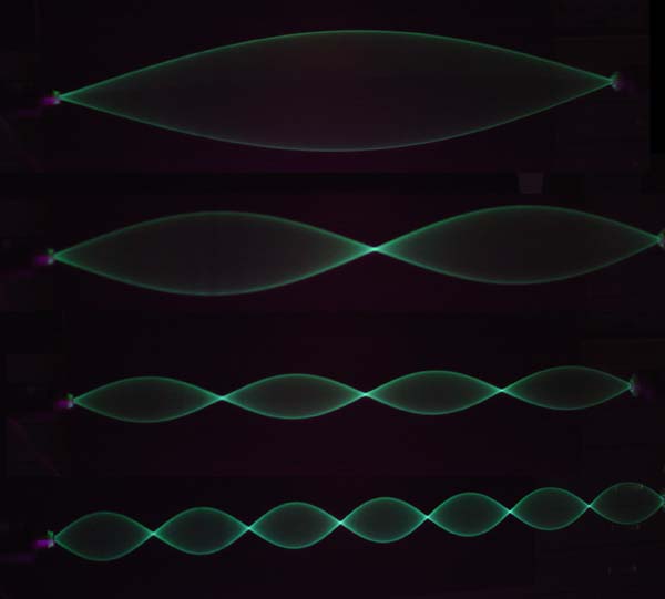
8. The mechanical driver will also vibrate a ten inch wire loop, and will induce standing waves with 3, 5, 7, etc. antinodes around the circle at specific increasing frequencies. Rudnick's String [33] shows the same effect on a linear string.
 |
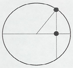
a. Analogy of Simple Harmonic Motion to Circular Motion:
A device which you crank around fits on a projector. One dot moves around the circle while another dot projected on a diameter stays underneath the first dot and executes simple harmonic motion. |
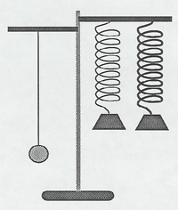
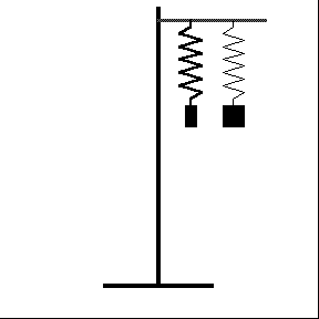
| b. Mass on a Spring:
Springs of two different spring constants are supplied along with several weights. A ruler device can be used with different weights on the springs to measure their k's. With a 200 g mass on the stiffer spring, the spring mode and pendulum mode are parametrically coupled. |
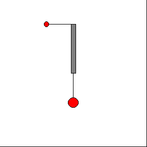
 |
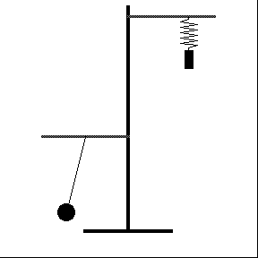
| c. Simple pendulum:
A simple pendulum is on the same device. You could also use the "Faith in Physics" Pendulum [2], or track a pendulum with a sonic ranger and plot out the sine waves of its motion (see Motion Concepts - Sonic Ranger [34]).
|
| d. Spring compared to Pendulum:
A pendulum whose length is equal to the displacement of a spring from equilibrium when the weight is attached has the same period of oscillation as the spring. |
 |
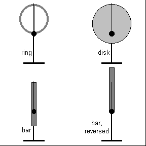 |
e. Physical pendula:
Each physical pendulum is compared to a simple pendulum with the same period. The bar can be reversed as shown, and has the same period in either position. |
f. Torsion pendulum: the weights can be moved as shown to change the rotational inertia, and therefore the period.

g. Coupled pendula: Three varieties are available.
h. Coupled gliders on an air track: Two gliders with three springs, two running to the fixed ends and the third between show normal modes and exchange of energy.
i. Some Unusual Pendula: Suggested by Bruce Denardo
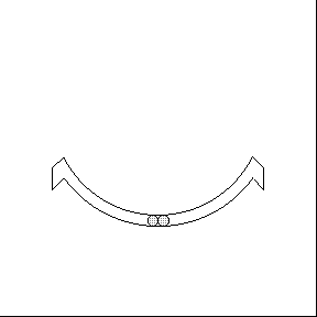
Simple pendulum, conical pendulum, collisions, Lissajous figures, and others can all be illustrated with this interesting demonstration. See Two Balls Hanging (Momentum and Collisions) [19]
 [19]
[19]
This is the famous torsional wave device. Among the concepts that can be demonstrated are:
A descriptive booklet is available.
See Doppler Shift (Acoustics) [37].
This demo illustrates the normal modes in standing waves. A black light shines on a motor- driven fluorescent string. As the input frequency changes and corresponds to one of the normal modes or harmonics, the nodes and antinodes appear. A strobe may be used to "freeze" a particular harmonic.
The Pasco Fourier synthesizer produces two 440 Hz fundamentals and eight exact harmonics. You can vary the amplitude and phase of any of these signals and add them up to generate a complex wave form. The output goes to an oscilloscope and also to a speaker so the class can hear the wave form. The two fundamentals can be added alone to show the sum of two sine waves, or sent to two speakers to demonstrate acoustical interference.
The Fourier analyzer shows the power spectrum of a complex wave form on an oscilloscope.
Applet by Fu-Kwun Hwang --- Virtual Physics Library [38]
How to play:
The default value for base frequency is f=100Hz, you can change it from the TextField (20 < f < 2000). The ear is 1000 times more sensitive at 1kHz than at 100Hz.
| frequency range | ||
| speech | song | |
| adult male | 80-240 | up to 700 |
| adult female | 140-500 | up to 1100 |
Can be illustrated with Moiré patterns on the overhead projector, or by adding sine waves of two different frequencies on the oscilloscope (M.P. Hagelberg, Am.J.Phys. 46(5),579 (1978)), or by showing a good film strip on the subject (#600).
Our large Kundt's Tube designed by Prof. Rudnick dramatically demonstrates standing acoustical waves. The speed of sound can also be measured. See Kundt's Tube (Acoustics) [39].
|
Further demonstrations that can be done with the Kundt's tube are described here [39] in the Acoustics section of the demo manual. |
A laser through various slits will project interference and diffraction patterns on the overhead screen. See Single, Double, and Multiple Slits [40].
A Russian wave machine separately models the motion of a string of beads undergoing transverse and longitudinal wave motion. The mechanism of its operation is almost more interesting than the effect it demonstrates.
Longitudinal and transverse waves can also be separately demonstrated by the Space Phone [41] and the Rubber Hose [42]. A slinky can be used to demonstrate both also.
 |
|
The 8D microwave lab setup can be used to demonstrate standing waves, interference, diffraction, polarization, and tunneling. A large lecture hall meter displays the output readings to the class.
Ultrasonic sound wavelength and interference can be demonstrated. See Acoustical Interference [43].
Stretches across the front of the lecture hall to illustrate standing wave modes. Strobes can be used to stop the motion.
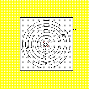
Our large ripple tank projects on the overhead screen to demonstrate reflection, interference, diffraction, etc.

Clamp a wave spring or rubber hose to the table and you can send a pulse along and see it reflected. The brass spring works best. Free end reflection can be accomplished by attaching a 1/2 meter long string to the end of the spring. If the end of the hose or wave spring is laid on the floor, you can send a pulse down and have it absorbed with no reflection.
is a longer, thicker string driven by a speaker. Hence, the driving frequency as well as the string tension can be varied. The equation v = (f/m)1/2 can be checked with either demonstration. This demo stretches across the front of the lecture hall to illustrate standing wave modes.
Vibrations of soap films on wire frames show various modes of oscillation.
This device can be used to demonstrate longitudinal and transverse waves. A pinch of the spring demonstrates a longitudinal wave and a pulse sent be flicking the wrist sends a transverse wave.
Metronomes of the same frequency and resting on the same base are started randomly. They synchronize after a short period of time. In this case the base is free to move. In 1657, Christian Huygens was the first to observe this phenomenon in the form of clock synchronization. The phenomenon of spontaneous synchronization is found in circadian rhythms, heart& intestinal muscles, insulin secreting cells in the pancreas, menstrual cycles, ambling elephants, marching soldiers, and fireflies, among others.
Two speakers are set a meter or two apart in front of the class. They are driven by an audio oscillator through a stereo amplifier at the same frequency, but the phase of one channel is variable with respect to the other, either using the circuit below, or the two fundamental channels of the Fourier synthesizer, Z.X.1. The phase is varied for the class so each student can hear the difference between constructive interference (loud) and destructive interference (soft). Then the phase is set at zero and all the students hearing a loud tone are asked to stand up, displaying the interference pattern across the lecture hall.
This demonstration occasionally produces erratic results in the lecture halls because of reflections from the walls. It works well in the anechoic chamber, but then you can take in only 10 - 15 students. A visit to the anechoic chamber and reverberation room would be very nice for a small class.
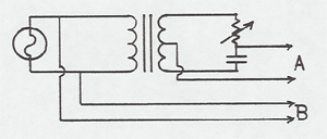
Ultrasonic Acoustical Interference - Small piezoelectric transducers (barium strontium titinate) resonate at 40KHz and can serve either as speakers or microphones. Two hooked to the same signal generator produce a very pretty interference pattern, which is read out by a third on an oscilloscope. Also the speed of sound can be measured by using one as a transmitter and a second as a receiver several centimeters away. The received signal is displayed on an oscilloscope synchronized to the transmitted signal. From the distances between phase coincidences and the frequency, the speed of sound can be computed.
Two tuning forks, one of which is adjustable in frequency, demonstrate beats. If the two tuning forks are adjusted to the same frequency and set next to each other, striking one will set up vibrations in the other.
There is a good computer demonstration of beats, which closely represents the tuning fork demonstration above. Two sources are created which play through the room speaker. The wavelength can be changed by dragging and the effects heard. At the same time, the beat waveform or the frequency spectrum can be viewed. This provides a couple different ways to visualize the beats.
The beat bars, tuned to 435 and 440 Hz, produce loud, definite beats. A strong effect is also produced by activating two Rijke Tubes of slightly different lengths. (See Rijke Tubes [46])
Another good demonstration beats consists of two audio oscillators hooked through a stereo amplifier to speakers. The summed signal is also sent to an oscilloscope so the wave envelope can be seen.
This standard demonstration which shows that sound is not transmitted by a vacuum has been improved by Prof. Rudnick. A sound transmitting seal over the vacuum jar has been provided so that the bell can actually be heard before the jar is evacuated. Circuitry built by R. Keolian rings the bell in bursts and simultaneously flashes a light so that the students can see that the bell is still ringing after the jar is evacuated and they can no longer hear it (and also note that light is transmitted by a vacuum, even though sound is not!).
Some have pointed out that this demo is not really what it seems. Sound travels very well in a poor vacuum, as long as the mean free path for collisions of air molecules is much less than the size of the container. For pressures achievable with the roughing pumps we use, about 1/10,000 of atmospheric pressure, the mean free path is about 1 mm. The speed of sound is proportional to the square root of the pressure divided by the density. Since the density is proportional to the pressure, the velocity of sound is independent of pressure.
So why does the sound diminish as the air is pumped out? It is a problem of the impedance match between the air and the bell and the air and the glass. The impedance of the air is proportional to the square root of the product of the pressure and density. Pumping out the air reduces the impedance of the air by a factor of 10,000 and the vibrations of the bell are not coupled to the air. If there was sound in the remaining air, it would not couple to the glass but instead be reflected at the interface.
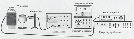
This demonstration requires a fair amount of equipment. A stereo amplifier, whose output goes to a horn driver near the wine glass to be broken, can be switched between a frequency generator, easily tuned through a broad spectrum, and a frequency synthesizer which can generate a?very accurate frequency. The response of the wine glass to the sound is monitored with a microphone connected to an oscilloscope. The first four steps can be prepared before the lecture, but most instructors like to run through them with the class so the students can see the entire operation.
We have the Tacoma Narrows Bridge collapse on videodisk. There is also a good online version which you can link to. The link is clickable Tacoma Narrows Bridge Story http://youtube.com/watch?v=ASd0t3n8Bnc [47]
The fundamental resonance of a wineglass is the bell mode which can be seen in the strobed video above. Two wavelengths of the resonant frequency fit around the rim, travelling in opposite directions, constructively and destructively interfering. There are four nodal points along the rim of the glass which don't move. In between the nodal points the glass walls are moving back and forth. Sometimes when the glass shatters it leaves evidence of the nodal structure as seen in the gallery below. The last two are rare breaks.
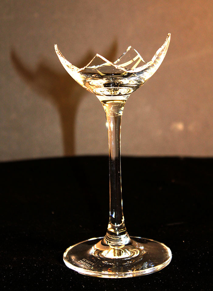
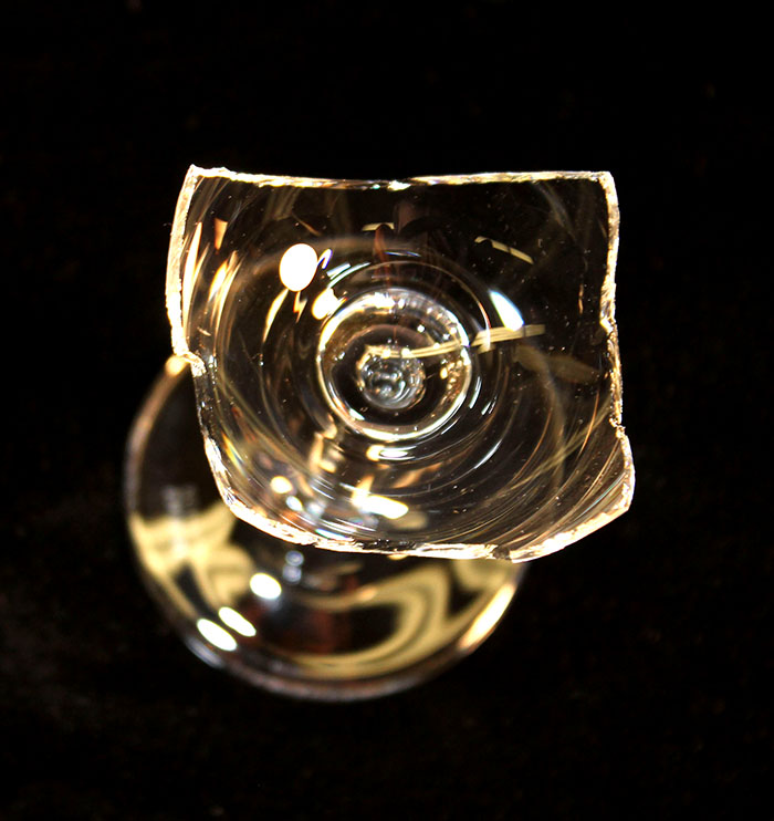
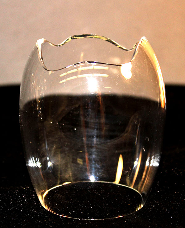
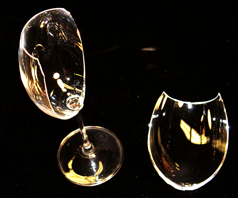
Exquisite patterns emerge from salt scattered on a metal plate which is stroked with a bass fiddle bow, illustrating two dimensional vibration. A video camera will enlarge the patterns for the class to see in the Knudsen lecture halls.
To form patterns, hold your fingers firmly on the nodes indicated, but try to localize them as much as possible. Use plenty of rosin on the strings and bow firmly. You are bowing on anitnodes; as you go from pattern to pattern, bow on a node of the previous pattern. That way you eliminate the previous one. a well bowed pattern gives a pure tone. And finally, practice, practice, practice!
Chladni patterns can also be formed by using circular or rectangular metal plates on a mechanical driver controlled by a signal generator. This method avoids having to practice your bowing. The patterns are now different since they have antinodes at the center (which is being vibrated) rather than nodes with the center rigidly attached and the edge bowed.
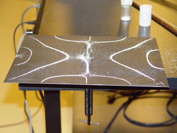 [49]
[49]
The Doppler effect for sound waves is dramatically demonstrated by swinging a ringing tuning fork around your head.
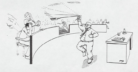
The whistle ball is another good way to demonstrate doppler shift. A sponge ball has been stuffed with a battery operated whistle in its core. As the ball is thrown around the lecture hall, the students hear a shift in the ball's frequency.
A sound clip is available indicating the doppler shift of a car horn at 30 MPH [50]. The link is http://www.exploratorium.com/imagery/sounds/30_MPH_doppler.au
The animated applet below is a good way to visualize the doppler shift. Click in the box below and then allow the applet to run. Click on the run button. You can control the speed of the source. The applet is also available on our ephysics site [51].
The picture below shows boat wakes which occur when the boat moves faster than the speed of water waves. Compare this to the ephysics applet when the source moves faster than the speed of sound.

Also dramatically demonstrates acoustical standing waves.
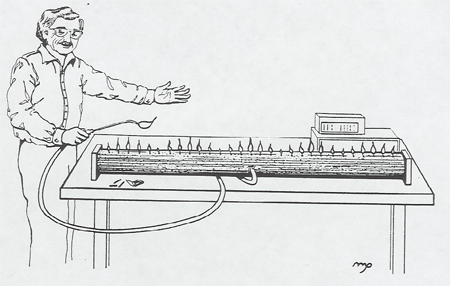
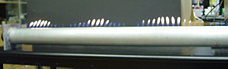
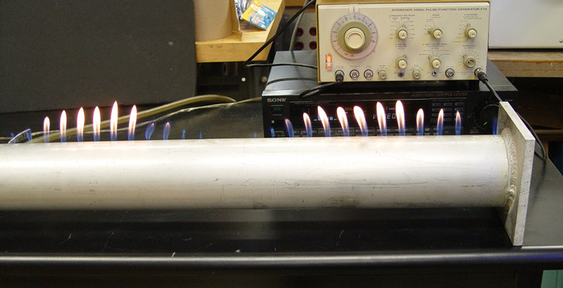
Small "balloon" flasks serve as Helmholtz resonators. When they are placed near a small speaker connected to an audio oscilator, the resonant frequency is very apparent as you tune through. The ejecting air will blow out a match. The resonant frequency will also be sounded if you blow over the opening as when producing a note from a bottle.
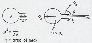

Our large Kundt's tube, designed by Prof. Rudnick, dramatically demonstrates standing acoustical waves. See the animation of standing waves [52] in the waves section of the demo manual. Additional demonstrations and accessories with this apparatus are:
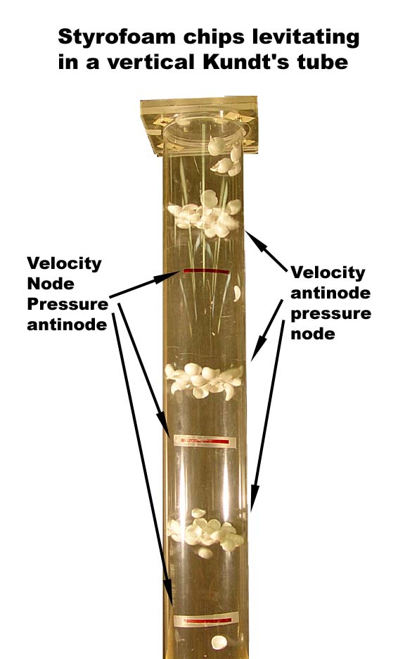
Several large metal tubes ROAR impressively when held vertically over Meker burners. The heat maintains the open-end acoustic standing wave mode (about 100 Hz).
A "Magic" Rijke tube has a wire gauze inside about one quarter the way from the bottom. Keeping the gauze concealed from the class, heat it red hot by holding it over a Meker burner on the floor. The tube will ROAR for some time after being removed from the flame from the stored heat. You can "tip the sound out" by tilting the tube horizontal, or block it by placing the lower end on the floor, and the ROARing will restart when the tube is vertical away from the floor if the gauze is still hot. Also, if you "tip the sound out", and then run across the classroom with the tube horizontal, bottom first, the ROARing will restart.
Heat up the magic Rijke tube, hold it away from the flame so it ROARS with the retained heat, and hold the normal tube over the flame. The tubes beat in their ROARing since, although they have the same lengths, they have slightly different diameters.
Rijke Tubes and Variable Stars
Similar to the standing sound waves exhibited in the case of the Rijke tubes, the pulsation mechanism for variable stars such as the Cepheids can be understood as a resonance of pressure waves of a particular period in the interior of those stars.
In the case of the Rijke tubes air can move in and out of both ends. A heated metal mesh placed a quarter of the way up from the bottom heats the air flowing past it. This flow of air is a combination of the convection current caused by the transfer of heat from the metal mesh and the sound wave that is set up for the condition of two open ends. For half of the oscillation cycle of the sound wave air moves in from both ends as it flows towards the center generating a pressure antinode (displacement node) there. Even though some of the air moving past the hot metal mesh has already been heated during the cycle prior to this, some additional cool air flows in, passing through it and acquiring thermal energy and further increasing the pressure, thus reinforcing the oscillation. For the remaining half cycle air passing by the metal mesh while flowing outward from the center of the tube is already heated and therefore energy transfer is minimal.
In the case of a Cepheid variable star, the partial ionization occurring in a He envelope allows for an increased opacity with increasing pressure, and is responsible for setting up the pulsation mode. The stage when the opacity is increasing corresponds to the part of the vibration cycle in the case of the Rijke tube when energy is transferred and the increase in pressure is amplified.
In both cases analogy can be drawn to an internal combustion engine.
Four small loudspeakers are used to excite standing waves in a plexiglass "room" 40 ¥ 40 ¥ 12 cm high. At 400 Hz one half wave fits in the 40 cm. About 140 dB of sound can be established in the "room". An audio oscillator feeds channels A and B through a stereo amplifier, but one channel is phase shifted 90° to the other. A reversing switch is provided to change the 90° "lead" to "lag". Thus, by using the balance control one set of speakers, or the other, or both, 90° out of phase, can be excited. By engaging the monaural mode the two signals are added, and both sets of speakers receive the same phase signal. A sample set of demonstrations is described below.
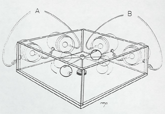
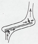
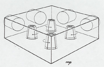
This record, produced by Bell Telephone Laboratories, (Folkways FX6136) is available on cassette tape. Single cuts can be played to the class.
Sound vibrations, compression and rare fractions: The Science of Sound has been recorded eight decibels lower than usual so that illustrations of acoustic phenomena can be presented with loudness approximately proportional to their level in nature. Adjust the volume of your phonograph so that the announcer sound as if he were speaking to you in a normal conversation voice. Then, orchestral music and certain other sound effects that would normally be louder than a human voice will sound louder.
The frequency range of the average human ear, sweep tone from 30 to 15,000 PCs.: This recording and the phonograph equipment on which you are playing it are, even more than your ear, limited in their ability to reproduce faithfully very lost and very slow sound vibrations. However, with high-fidelity equipment, you may be able to hear vibrations between about 50 and 12,000 cps. The sweep frequency tone is recorded according to the recommendations of the RIAA. Playback equipment that is equalized for the RIAA curve and operating correctly will reproduce all tones from your loudspeaker with approximately equal power. Differences in the apparent loudness of the various frequencies are due to the characteristics of the human ear. These pitch versus loudness characteristics have been charted by Fletcher and Munson and can be seen in most standard textbooks on sound and acoustical engineering.
How pitch depends chiefly on frequency and is some extent on loudness the subjective nature of pitch: the mel scale. the standard reference for 1000 mels is a 1000 cps tone at 40 decibels above 0.0002 dynes per square centimeter. the mel scale tones on this record are presented at greater intensities so that they can be heard more easily.
Measuring sound intensity; standing waves; the decibel: The average human ear has a maximum range of about 130 decibels between the threshold of hearing below which no sound can be heard, and the threshold of feeling, above which sound intensity becomes uncomfortable. Since the range of ordinary phonographs is limited we have not attempted to demonstrate an intensity range of more than about 40 decibels.
Two instances of the Doppler Effect: (1) observer moving, sound source stationary;(2) observer stationary, sound source moving. (the sounds of racing cards were recorded at the 1956 International Sports Car Grand Prix, Watkins Glen, N.Y.).
Speech accompanied by echo from reflecting surfaces at 500 ft., 200 ft., and 50 ft: How speech sounds in rooms with long, moderate, and short reverberation times. This demonstration was produced in Bell Telephone Laboratories by means of magnetic tape delay devices in combination with a reverberation chamber. So that delay differences could be heard easily, the echoes are recorded somewhat louder than generally experienced. An attempt is made, however, to present the loudness of an echo in accordance with the length of the echo path.
Speech and music with some frequencies delayed in transmission: This demonstration was simulated by using a delay system with multiple recording heads located around a rotating magnetic disc. the sound is split into two bands by high-pass and low-pass electronic filters that have a cross-over frequency of 3000 cps. (The music is a trumpet fanfare by Semmier.)
The fundamental; overtones; harmonics: The lowest frequency present in a sound is called the fundamental, frequencies high than the fundamental are called overtone frequencies. A special tone generator developed at Bell Telephone Laboratories was used to produce the various tones used in this demonstration.
The effect of overtones on sound quality: A factory whistle, a soprano, and a piano are compared with and without overtones. Special low-pass filters with unusually steep slopes of cutoff (150 decibels per octave) were used in this demonstration to eliminate some overtones. Attenuation in the stop band is 55 decibels or greater.
Music and speech with various frequency ranges eliminated: The filters that were used in this demonstration have sharp cutoffs. 250 decibels per octave. Attenuation in the stop bands was 55 decibels or greater. Wedding Day at Troldbeugen by Greig is played by the Bamberg Symphony Orchestra.
The speed of sound is given by v =rad(gp/p). Since the density p is proportional to the molecular weight A at STP, then v = 1/ rad(A) for monatomic gasses. (In comparing with air we also have to take into account the different g.) For a light gas like helium the speed of sound is higher, and more wavelengths can fit in a fixed distance like an organ pipe or human voice box. The pitch is therefore raised by this same factor 1/ rad(A), about 3 for helium. You can breathe some helium and demonstrate the Donald-Duck-like effect, or blow some into an organ pipe to raise its audible frequency.
What gas shall we use to lower the pitch of the voice?- a gas of high molecular weight, but another most important property is that it be non-toxic. Some possibilities are listed below:
| Gas | Molecular weight | Approximate price for 1 mole (22.41) at 99.995 purity |
| helium | 4 | $1 |
| air | 29 | free for now |
| krypton | 84 | $228 |
| xenon | 131 | $550 |
| radon | 222 | trace quantities supplied free in some municipalities |
| sulfur hexafluoride | 146 | $4 |
Radon is the heaviest gas, and, chemically it is completely inert. However, since its longest lived isotope has a half?life of only 3.8 days, sulfur hexafluoride is the gas of choice. This gas is colorless, odorless, tasteless, water-insoluble, thermally stable, non toxic, and non-reactive. As shown in the diagram, the six fluorine atoms completely surround the central sulfur atom protecting it from attack. The strongly electronegative fluorine atoms make this gas very difficult to ionize. It is a much better gas-phase insulator than air; thus, it is used in high voltage electrical switches. You might wish to demonstrate the heaviness of this gas by filling a balloon and then throwing the "lead balloon" across the room.
Our formula above predicts that the speed of sound in sulfur hexafluoride is about half as fast as in air, so the pitch is halved.
Lecture bottles of He are available for demonstration. It is a good idea to allow some breathing space between the demonstrations to make sure you keep getting plenty of oxygen.
Ultrasonic Xylophone - range from the high audible frequencies into the ultrasonics.
Galton's Whistle - range from the high audible frequencies into the ultrasonics.
Organ pipes - one is of variable length to show the dependence of frequency on length.
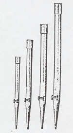
Sicks - You can play a tune with a set of eight sticks tuned to the major scale by dropping them in the correct order.
Singing tube - when whirled around your head will sound the notes of a major chord.
Siren disk - has four evenly spaced rows of holes yielding a major chord when sounded. The fifth row is unevenly spaced and emits a noise when sounded.
Savart's toothed wheels - will sound a major chord when rotated with a card held against its teeth.
Ultrasonic Receiver - beats ultrasonic signals from a speaker "tweeter", or the Ultrasonic Xylophone (e) or Galton's Whistle (f) in the 20-40 KHz range into audible range.
Music Box - Each tine of the box acts as a simple harmonic oscillator and vibrates at a particular constant pitch. The pins on the box pluck the tines to make them vibrate but the tines alone don't emit much sound. To project sound, the box couples its vibrating tines to a surface.
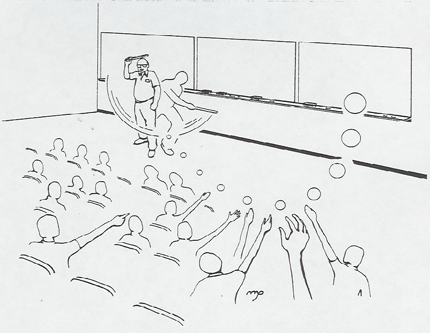
A very simple demonstration is to attach a one kilogram mass to a spring scale and lower the mass into an aquarium of water. The weight under water is considerably less than the weight in air.
We have a much more elaborate apparatus with two large produce-type grocery scales, one over the other. The lower one holds a pan of water, and the upper one weighs a mass in air or in the water. You can measure the dimensions of the mass, compute the volume it displaces, weigh it in air and in water, and note how the weight of the pan of water changes when the mass is lowered into it.
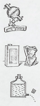
Several short demonstrations nicely illustrate Bernoulli's principle.
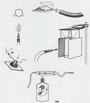
In a container of water sealed with a rubber diaphragm top is a smaller floating container partially filled with water and with a small hole in the bottom. When the rubber diaphragm is depressed, the air in the smaller container is compressed, increasing the volume of water in the smaller container and reducing its buoyancy. Thus, the smaller container sinks. Its level can be controlled by the finger pressure on the diaphragm.
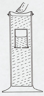
Water is added to a connecting set of tubes with progressively smaller bores. Capillary action raises the water progressively higher in the smaller bores.
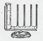
A bell jar with several demonstrations is evacuated in class:
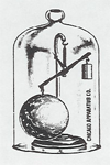
A container has four immiscible fluids floating, one above the other - mercury, carbon tetracloride, water, and naptha. You can lower in small cubes - balsa, hardwood, plastic, and aluminum - to float at each interface.
Demo 1
A manometer with a rubber diaphragm-covered probe and an aquarium filled with water and a marked level of depth are provided. The pressure probe is inserted under the water to the marked level of depth and faced up, down, and sideways. The pressure reading is the same for all directions.
Demo 2
Pressure Syringe (aka Pascal's Demonstrater) Fill the syringe with water, push the plunger, and watch the water shoot out of every hole equally.
Corn starch and water are mixed in a plate to produce a goopy mixture that can be scooped up and dribbled with a spoon. Inviting the students to look closer, the professor suddenly slams his or her fist down on the mixture, causing the students to jerk back - but the mixture doesn't splatter; it momentarily becomes rock hard when acted on by a large force. Another type of behavior is demonstrated by dragging a spoon rapidly through the mixture to cause a ripping action.
Also available is "silly putty" which is hard and elastic under large forces but flows under small forces. Mold it into a ball and bounce it, and then leave on the lecture table; in ten or twenty minutes it will flow out under gravity.
A set of tubes of different shapes are connected to a common source of water. When filled, the water reaches the same level in all the tubes.
This is a demonstration that pressure depends on depth only and not on the shape of the vessel. The reservoir on the right is adjusted for the same level of fluid in each "vase", and the gauge reads the corresponding pressure.
With a right-angle plywood trough covered with sandpaper, you can put a tremendous curve on a ping-pong ball, even curving upwards from a horizontal throw.
Suggested by Prof. D. Pursey from Iowa State, who is shown above in action.
A can has openings one quarter of the way down, one half of the way down, and three quarters of the way down. When filled, water flows out the openings. From which hole will the stream impact furthest from the bottom of the can?
Bottles of water and glycerin have similar beads in them which sink at different rates according to the viscosity of the fluid.
The Fire Syringe demonstrates an adiabatic process. The autoignition temperature of cotton is 407oC (765oF).

A thin piece of pyrolytic graphite cuts through an ice cube. This material, of layered graphene, has excellent electron and thermal conductivity along the layers, but poor conductivity through the layers. This made it good heat shielding material for re-entry vehicles. It's diamagnetic properties are also anisotropic, with a very strong response to fields perpendicular to the layers.
Identical small balls are attached by wax to the ends of six rods of different metals, radiating from a common metal center. The center of the rods is heated with a flame, and the small balls drop off at different times as the heat is conducted out by each different rod to melt the wax holding the ball.
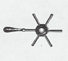
Drinking Bird - The bird dips its beak into a beaker of water "taking a drink" and rotates back up. Cooling by evaporation from its beak draws up a colored liquid (methylene chloride) through a tube in its body overbalancing the bird so it takes another drink. This action repeats indefinitely.
Love Meter - Hold this device in your hand and heat from your hand boils methylene chloride causing it to flow through an intricate series of tubes.
See also Galileo's Air Thermometer [55]
How can you walk across hot coals?
Firewalking has been going on all over the world for thousands of years with written records going back to 1200 BC. Eastern Orthodox Christians in Bulgaria firewalk during popular religious feasts. So do Japanese Taoists, Buddhists, Indian Fakirs, the !Kung Bushmen, Polynesians, etc. Some claim that firewalking is an example of mind over matter, or a test of the protective power of faith.
It is true that the temperature of the coals is over 1000 degrees F (535 degrees C), and that human flesh burns at much lower temperatures, but temperature isn't the only part of the relevant physics. It wasn't until the 1770's that Joseph Black figured out the relation between thermal energy and temperature. (He later discovered Carbon Dioxide.) Different substances have different heat capacities. Water is the standard. It takes 4.18 Joules to raise the temperature of 1 cc of water 1 degree C. Our feet are mostly water. The coals have a much lower heat capacity than water. That means that the same amount of energy flowing away from the coals will lower their temperature much more than that same energy flowing to the feet will raise the foot's temperature. If the foot stays in contact with the coals, energy will keep flowing until they both reach the same temperature. However, this takes time, and how much depends on the heat conductivity. There are good heat conductors, like water, and poor conductors/heat insulators, such as ash. The feet cool down the local area of the coals they touch, and it takes time for energy to flow from the rest of the fire to the cool spot. You can sometimes see dull orange footprints in the coals right after someone walks. Water is a good heat conductor and energy transferred to the foot is rapidly conducted away from the contact points so the temperature doesn't rise to the burning point. Temperature, heat capacity, and thermal conductivity are all important in this demonstration.
A more familiar experience which involves the same physics is baking brownies in the oven set to 450 degrees F. Everything in the oven is 450 degrees, but you don't fear putting your hand in the oven air. The air has a very low heat capacity meaning it stores very little thermal energy. Air is also a heat insulator. Your hand (mostly water) cools the air locally and heats up very little. If you stick your finger in the brownie, you might get burned. It is mostly water like your hand and has a pretty good heat conductivity. Thermal energy will flow to your finger raising its temperature quickly. The metal pan is another matter. It has a high heat capacity and a high conductivity. Touch it without a potholder and you might instantly burn your fingers.
What the physics tells you, is that if you walk fast and don't stay in contact with the coals very long, you won't get badly burned. If you believe in mind over matter or the protective power of faith, then time shouldn't matter. This could be a life threatening delusion.
Even knowing the theory, firewalking is still dangerous in practice. There is a lot of energy in a glowing firepit at 1000 degrees F. Second degree burns in the form of blisters are common and more severe burns requiring a trip to the hospital have occurred. Sometimes a hot coal will stick to the foot causing a burn. There can also be hot spots in the fire, pieces of metal, or even pockets of hot steam locked up in the wood. Falling down in coals can be fatal. We will take care to make our walk as safe as possible.
Watch a video explanation of firewalking [56]. The video includes comments from Bernie Leikind, who got his start firewalking at UCLA.
One last note: Just because some aspects of firewalking and heat are "just physics", don't try to copy any fire stunt you might see. There have been many fire performers throughout history who used trickery to amaze audiences, and if you tried to duplicate their trick you would be severely injured. For instance, some performers scooped boiling lead into a ladle, and then poured it into their mouth. Shortly after, they spit out a chunk of cold lead with their teeth impressions in it. However, all was not as it seemed. The ladle had a hollow handle with mercury inside. Instead of scooping molten lead, mercury from the handle filled the ladle. Instead of pouring molten lead in their mouth, the mercury just went back into the handle. The cold lead with the teeth impressions had been hidden in the mouth beforehand.
In order to get liquid nitrogen we need a little extra notice. Some experiments are:
| Gas | In atmosphere | Boiling point | Melting |
| Nitrogen | 78.1% | 77 K, -196 C, -320 F | 63 K |
| Oxygen | 20.9% | 90 K, -183 C, -297 F | 54 K |
| Argon | 0.9% | 87 K, -186 C, -303 F | 84 K |
| Carbon Dioxide | 0.038% | 195 K,-78 C, -108 F | none |
| Helium | none | 4.2 K, -269 C, -452F | 0.95 K |
A flask of air connects at the bottom to a column of water. When the flask is heated by your hand, the air expands and the water falls. When it is cooled by evaporating alcohol, the air contracts and the water rises. Why doesn't this make a good thermometer? (It also responds to barometric pressure.)
What does the energy locked in 1 gram of sugar, 16 kilojoules, look like? Let's oxidize a gram and see.
This is an example of an exothermic reaction. The white powder is Potassium Chlorate. When melted it becomes a source of reactive oxygen. A typical gummy bear is 1 gram of sugar. Glucose + Oxygen ⇒ Carbon Dioxide + Water + energy
C6H12O6 + 6 O2 ⇒ 6 CO2 + 6 H2O + 16 kilojoules per gram of sugar
In cellular respiration sugars are oxidized and the resulting energy is stored in molecules of ATP. Each gram of sugar produces about 3.75 kilocalories or 16 kilojoules of food energy. The average human body utilizes about the same energy as a 100 watt light bulb. 100 watts x 24 hours x 3600 seconds/hour = 8,640 kilojoules per day. (Starvation is considered to be less than 1800 kilocalories or 6,830 kilojoules per day.) If we got all our energy from sugar and starch, we would need about 540 grams/day which is just over 1 pound per day.
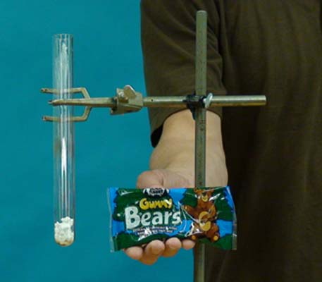
If we could power our bodies with electricity from the utility it would take 2.4 kilowatt hours to operate at 100 watts for a day. At the rate of about 10 cents per kilowatt hour, the energy would cost 24 cents.
For more details on cellular respiration from the Khan Academy:
A set of five balls of different metals is heated in boiling water. The balls are then dropped onto a thin paraffin slab. They melt their way through at rates depending on their heat capacity (which depends on both the specific heat capacity of the metal and its mass).
Dissimilar metal wires with two junctions are hooked to a galvanometer. Heating one of the junctions with your fingers produces a substantial reading.
A steel ball bouncing on a polished steel mirror illustrates a highly elastic case; the ball will bounce for a considerable time.
With another piece of apparatus balls of different materials can be bounced on steel. Some (glass, steel) are highly elastic, and some (wood, lead) are highly inelastic. The bounce height can be measured approximately with the apparatus.
Nine basic crystal lattice models [58] are available including face-centered and body-centered lattices [59] and Bravais lattices [60].
See Imiscible Fluids [61]. Four immiscible fluids float one above the other - mercury, carbon tetrachloride, water, and naphtha. Small masses - aluminum, plastic, hardwood, and balsa - lowered into the fluids float at the four interfaces.
A face centered
and body centered lattice are available.
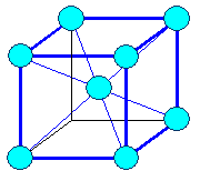
Bravais demonstrated that there are fourteen different point lattices, shown below in a sketch and photograph.
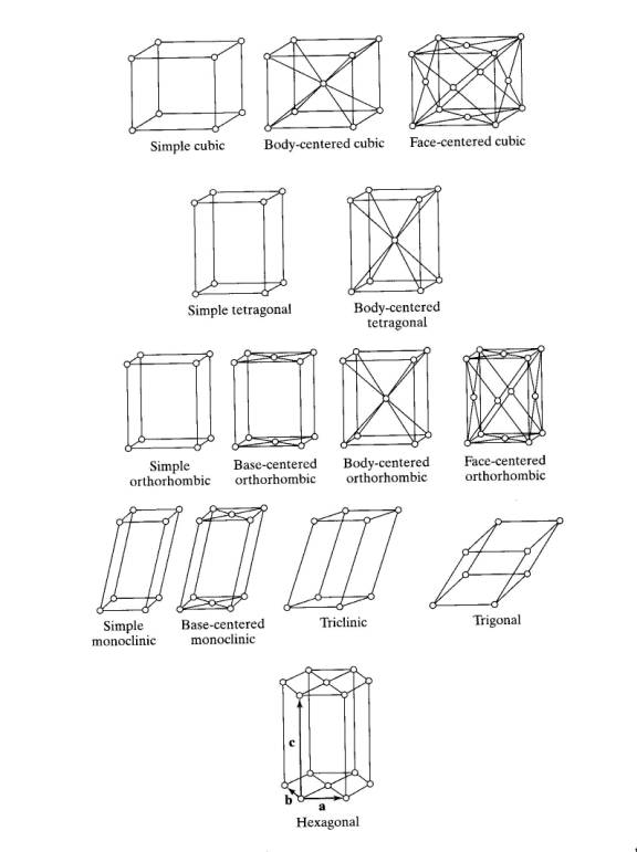
The following basic crystal lattices are available for demonstrations.
A large Pyrex flask of water is heated to boiling; then the flame is removed and the flask sealed off. When water is poured over the flask, cooling it, the steam in the flask condenses reducing the vapor pressure, and the water boils at the lower temperature.
Smoke is drawn into a small chamber and examined under a microscope to observe Brownian motion.
Another demonstration for Brownian motion is an apparatus which gets placed on the overhead projector. Balls of different size can be used to show the random motion of molecules. As the speed on the agitator is turned up, the balls move faster.
Lastly, an ephysics applet [62] for Brownian motion is available on the web.
See Effects in a Vacuum [63]. Water boils at room temperature as the air above it is evacuated. Its temperature as measured by a thermometer drops rapidly. The more elaborate demonstration in which water is frozen in this way requires the addition of a beaker of concentrated sulfuric acid to the vacuum chamber to further reduce the vapor pressure.
A thermoelectric device which runs a propeller has two legs. The device will run if one leg is in a hot cup of water and the other in a cold cup of water, but not if both legs are in the same cup of water. (The hot and cold water can be mixed for the second step to show that the ability to do work has been lost.)
The "Thermobile" will spin (by shape-memory retention) if one end is dipped in hot water. Air at room temperature serves as the other reservoir (also see Laws of Thermodynamics [64]).
A spinner rolls indefinitely up and down a double ramp. Is this perpetual motion in violation of the First Law?
A Hilsch tube device connected to the room air source separates the air stream into hot and cold blowing streams. Does this violate the Second Law?
The "Thermobile" runs when dipped into hot water. Is this a heat engine with only one temperature reservoir?
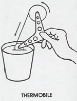
The thermoelectric converter can also be run between ice water and liquid nitrogen demonstrating that there is still plenty of heat energy in ice water.
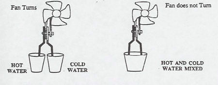
Professor Izzy Rudnick's 17-minute film on effects in liquid helium dramatically shows superfluity, fountains, super leaks, etc. and discusses the thermodynamic functions and properties of liquid helium.
A motor-driven molecular motion model which rattles various sized ball bearings around wildly fits on an overhead projector. The model also contains a somewhat larger object which is jiggled by impacts from the balls to demonstrate Brownian motion.
With this apparatus, a ball is bounced on air. From the period of oscillation the ratio Cp/Cv can be calculated. Instructions and method of calculation are available.
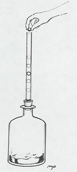
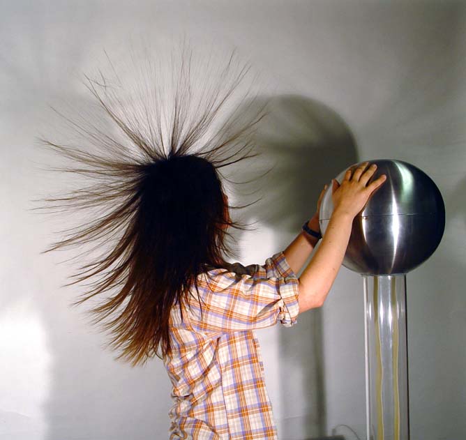
A light bulb with a large curly filament is connected alternately to 110 V AC and DC sources. A magnet is brought near the bulb. The filament under goes a steady deflection in the case of DC, but vibrates impressively in the case of AC.
The difference can be further illustrated by hooking a large inductance or capacitance in series with the bulb. The inductance "passes" DC but "blocks" AC, whereas the capacitance "blocks" DC but "passes" AC. See Capacitors and Inductors [65] for details.
Here is another demonstration of AC: A bicolor LED is connected directly to the 110V AC line. When the instructor swings the LED around her/his head, the light flashes green then red, showing that the LED is lit for only one half of the AC cycle. The same LED can be connected to a DC source, then the LED has one polarity, either red or green.
- This is a circuit that looks very much like the canonical series circuit, but the switches and lights don't do what's expected. There has to be a deeper level of knowledge and understanding to figure it out.
Here's the apparent circuit.
The puzzle is, what components can be added to this circuit to give the observed behaviour? One could think about the effects of common components such as resistors, inductors, capacitors, diodes, transistors, etc. I can tell you it doesn't involve magnets or radio frequency transmitters. If you figured it out, check the solution. If you haven't, I can give you three hints:
Diodes provide the coding and decoding by phase of the AC current. A diode is put in parallel with the each switch and light.
A diode is a uni-directional valve. It will let current pass in one direction but not the other. A diode in this direction  will let positive current pass from left to right but will block negative current. From the other direction negative current will pass but positive current will be blocked. Diodes are marked with the vertical bar to indicate the direction.
At the switches:
When the switch is open, all current is forced to flow through the diode. One switch diode blocks positive current and one blocks negative current. If both switches are open, all current is blocked and no lights light up.
When a switch is closed, the diode is bypassed, shorted out, and both polarities can pass through the switch. Otherwise, each diode blocks one polarity.
At the lights:
The lights act as resistors and will pass both polarities. Here, each diode acts as a short circuit for one polarity, and acts to bypass the light. The other polarity, blocked by the diode, is forced through the lamp and causes it to glow.
With two switches there are 4 possibilities:
open open 0 current
open closed + current
closed open - current
closed closed + and - current
One light turns on from the + current and one from the - current.
Here's a circuit where the lights are replaced with led's. See if you can figure out what should happen.
Various low-pass and high-pass RC and RL filters can be constructed to your taste. The Pasco Waveform Analyzer has tunable low, high, and band-pass filters built into its circuitry so the harmonics of a square, sawtooth, or other complex waveform as from the Fourier Synthesizer, can be analyzed.
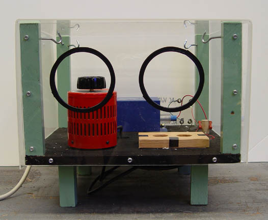
A simple RC circuit will integrate or differentiate waveforms:
(Of course, the derivative and integral of a sine wave is the leading and lagging cosine wave; these are just the normal 90° phase shifts.) The circuit below integrates.
The resistance R is made large and the capacitative reactance Xc is made small by using a large C and/or a large W. Then the current into the circuit is set by R and proportional to Vin. The capacitor stores and integrates the charge.
To differentiate the circuit is wired as below:
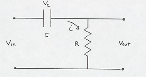
We arrange for nearly all the input voltage to drop across the capacitor (Vc >> Vout ) by making R small and Xc large using a small C and/or w Thus the voltage drop across R measures i without disturbing Vc.
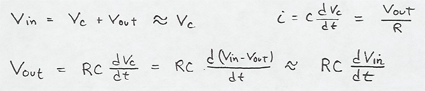
The circuit looks essentially like a capacitor to the input. The current is set by C and the small R is placed in series to sense it. RL circuits will perform the same operations.
A relaxation oscillator circuit as seen in RC Time Constant [67] demonstrates the RC time constant by a flashing neon bulb.
With a square wave input the voltage across the capacitor shows the exponential decay on an oscilloscope.
You could roughly measure the time constant t c= RC from the oscilloscope trace. With a similar circuit for RL you could estimate the time constant tL = L/R. These circuits are analyzed and their oscilloscope traces depicted in Halliday and Resnick, Part 2; for RC, Section 32-8, pp 705 -709; and for RL in Section 36-3, pp 798 - 801. As discussed in E.7.5, the same circuits will integrate and differentiate waveforms.
A simple, graphic demonstration of a series RLC circuit is to use a small light bulb for the R. Then you can tune through resonance and see the bulb's brightness reach a maximum, or you can set the frequency a little below resonance and insert an iron core into the inductor and see the bulb's brightness go through a maximum.
A parallel RLC circuit is set up so it can be driven with a signal generator and its resonance observed on an oscilloscope. The R (and thus Q), L and C are all variable. Alternatively, the circuit can be pulsed and the exponentially damped oscillations observed on a scope.
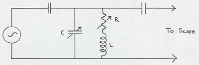
(The small input and output capacitors serve to isolate the RLC circuit.)
If the signal generator is replaced with a sweep frequency generator, the oscilloscope can be caused to actually draw the resonance curve.
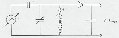
The sweep generator repeatedly sweeps across a band of frequencies including the resonance. The output of the RLC circuit is then amplitude modulated by the resonance curve. Its average is still zero, but after passing through the diode which acts as a detector and being smoothed by the capacitor the final result is the response curve of the RLC circuit as a function of frequency. You can vary the position of the peak of the curve by changing C or L, or you can vary the width of the curve (Q) by varying R.
You may become confused when you try to use the dual trace feature of the scope, for example, to demonstrate the 90° phase shift of a capacitor, unless you understand how the leads are grounded.
One side of both scope leads is grounded, and one side of the signal generator is grounded. This prevents you from hooking up the naive circuit below to show the 90° phase shift.
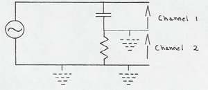
You can "fake" the situation by using a small resistor (1000W) as shown below.
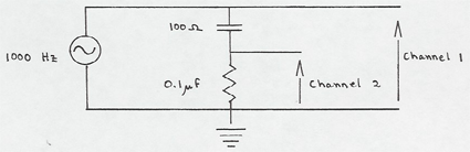
The voltage across the resistor alone shows the phase of the current through the capacitor. The voltage across both is the voltage across the capacitor -- mostly, if R<< Xc. Then these two voltages are almost
90° out of phase. For a capacitor, then, you want to use a low frequency so Xc is large.- In the similar circuit with an inductor you would use an high frequency so XL is large.
But the simplest way of demonstrating the same phase shift is use a two prong adaptor on the plug of the signal generator. Then the signal generator ground is floating, and the circuit can be hooked up as below.
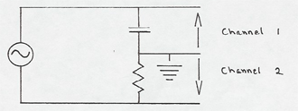
You are reading the voltages across the resistor and capacitor in the opposite directions, so press the invert button on channel 2 of the scope to show properly that the voltage lags the current in a capacitor.
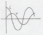
Adjust the two signals to have the same amplitude, and then turn the sweep rate knob counter-clockwise to the X-Y position to display the 90° phase shift in the form of a perfect circle.
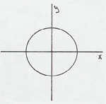
The similar situation with an inductor is well shown with L = 50 mH and R = l0K.
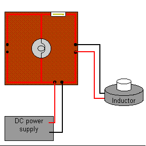
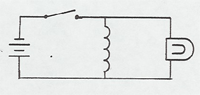
The voltage in the circuit above is adjusted so that the light bulb glows dimly. When the switch is opened, the bulb will flash much brighter momentarily as the magnetic field collapses around the inductor.
A neon bulb can be substituted and the voltage adjusted far below threshhold. The neon bulb will flash when the switch is opened, showing that the back EMF is much larger than the steady voltage.
The circuit can be arranged to produce a large spark when the switch is opened.
Impressive sparks are produced when various capacitors are discharged.
A 4000 F capacitor is charged to 150 V. It can then be carried close to the class and snapped in front of them. This is guaranteed to wake up the sleepers!
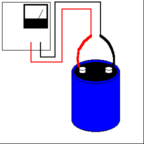
A Leyden jar is charged to 50,000 V with a Van de Graaff generator. It can even be disassembled and the outer and inner cans touched together, and then reassembled (carefully! ). Now, when the outer and inner cans are bridged by a discharge wand, a half-inch spark jumps. (See E.1.5 [68]).
 |
 |
Wire exploder: A 175 F capacitor is charged to 4000 V and discharged through a small wire. The wire vaporizes with a large bang and flash. This demonstration is dangerous and must be performed by a lecture demonstration staff member.
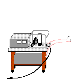
Sources of 110 V AC and DC are fed alternately to a standard incandescent bulb in series with a large inductance or capacitance. The capacitance will "pass"AC but "block" DC, whereas the inductance will "block" AC and "pass" DC. With the AC supply, if an iron core is lowered into the inductor coil, increasing its inductance, the light bulb becomes dramatically dimmer, illustrating a theater light dimmer circuit.
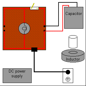 |
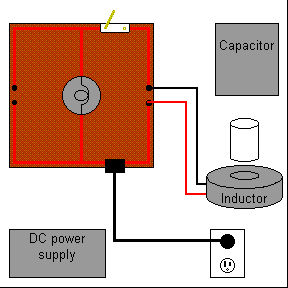 |
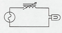
This apparatus is based on a fusion energy device called a theta pinch. A large capacitor is charged and a high current switch discharges it through a coil with just a few turns. The "theta" current in the coil produces a radial pinching effect on any conductor inside the coil.
In the can cutter variation, an empty aluminum can is pinched in the center and shoots out both ends. In the coin shrinker version, a coin is placed inside a sacrificial coil and a blast shield is used. The coil blows apart into pieces of molten wire, leaving behind a shrunken quarter.
There are a couple ways to explain what happens. The first is to look at the eddy currents induced in the conductor, and then noting that the I x B forces are radially inward. Or, it can be treated as the force between antiparallel wires. Another way is to look at the magnetic energy which goes as B^2 and the magnetic pressure which is the gradient of B^2. The discharge happens on an RC timescale but the magnetic field penetrates the conductor in an L/R time. Before the field can penetrate there is a large gradient in the magnetic energy trapped between the conductor and the coil and this results in a radially inward force.
The current and instantaneous power in this device is enormous. The coin shrinking happens in about 40 microsec. The current is about 60,000 A and the power (during the discharge) is 360 MW, as much power as a small city uses for that instant.
Magnetic pinch technology is used for industrial metal forming. Thin tubes are crimped or welded and metal sheet can be magnetically pressed into a form.
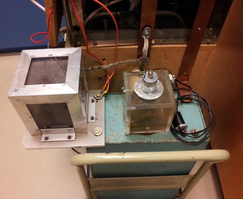
The 4000 F capacitor above is charged to 120 V. If it is discharged by shorting the wires, a bang and flash results. But you can also connect it to a 20 watt light bulb, and the stored charge will light the bulb for several seconds.
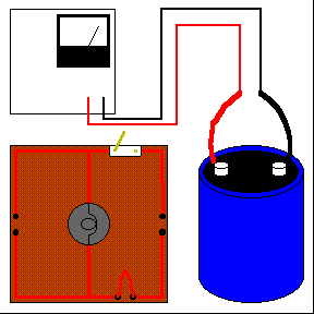
A Leyden jar is a capacitor consisting of a glass can with aluminum foil inside and outside, which can be charged up to several tens of thousands of volts with an electrostatic generator. The jar will retain the charge for many minutes, showing charge storage by a capacitor. The jar can be discharged by bridging the inner and outer conductors with an insulated discharging wand and drawing a spark.
The Wimshurst generator [69] has Leyden jars that can be connected in or out of the circuit, illustrating several aspects of capacitors.
See also the Dissectible Leyden Jar [68].
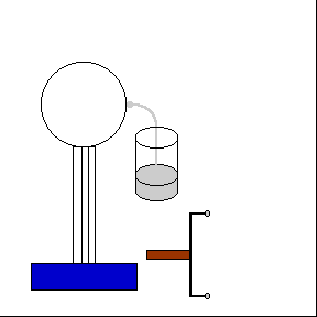
A parallel plate capacitor has variable plate separation.
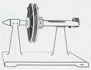
Some interesting demonstrations are:
a. The capacitor is connected to an electrostatic voltmeter. It is charged to one thousand volts with a high voltage supply. (The high voltage supply is in series with a lOOMohm resistor so its leads are safe to handle. The capacitor will be discharged in an instant if you put your fingers across the plates. Nothing will be felt; the stored charge Q with this capacitor is too small to make an appreciable current.) With the capacitor charged and disconnected from the power supply, the plate separation is now increased. Ask your students whether the voltage across the capacitor as shown by the electrostatic voltmeter will increase, decrease, or remain the same. Similarly, with the capacitor charged and disconnected from the power supply, a dielectric is thrust between the plates. Will the voltage increase, decrease, or remain the same?
 |
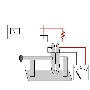 |
b. A measuring amplifier can be inserted into the charging circuit from the high voltage power supply. Even after the capacitor is charged a slight leakage current will be noted. You can grasp the plates with your fingers, and the additional current flowing through your hand (protected by the l00Mohm resistor) will be noted on the meter. If the plate separation is increased, additional current will flow in to increase Q. A dielectric thrust in produces similar results.
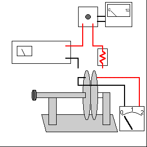 |
 |
In the "unitary imbecilometer" circuit the capacitor C charges slowly through the resistor R. When the voltage across C reaches the threshold of the neon light N (about 90 V), the capacitor discharges through the bulb, flashing it, and the cycle repeats. The frequency of flashes can be varied by varying R or C.
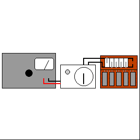
Zinc-copper-acid battery. Cut-away dry cell Batteries in series and parallel can be demonstrated.
Lemon cell - a copper and zinc nail pushed into a lemon will produce about 0.9 V on a meter. Two lemon cells hooked in series will light a small red led. Bring your own lemons.
Electrolysis of water apparatus is shown in the video below. NaOH is used as the electrolyte. The gasses are tested in the second video. Oxygen will relight a smoldering wood splint. Hydrogen causes a small pop when ignited.
The internal resistance of the Leybold multimeter on the 10 V scale can be measured with the circuit below:
The ammeter reads the entire current flowing through the internal resistance of the voltmeter, and the voltmeter reads the voltage drop across this resistance, so ri = V/i. You can check this by inserting a resistance decade box in series with the circuit and adjusting the resistance until the meter readings go to one half their former values. The decade box will then read the internal resistance of the voltmeter (assuming that of the ammeter is much smaller).
One way to measure the internal resistance of an ammeter is the circuit below.
The decade box R2 is set to zero, and R1 is chosen for an approximate full scale reading for the ammeter. R2 is then adjusted to halve this reading, so its resistance equals that of the ammeter.
ri for Leybold multimeter on 10 V scale = 34,000 ohms
ri for Leybold multimeter on 1 mA scale = 120 ohms
ri for Leybold projection meter on 1 mA scale = 100 ohms
A hot dog is impaled on nails connected directly to the 110 V AC line; alternatively DC can be used. Current passing through the hot dog will cook it in a minute or two. You can make the demonstration dramatic by putting the cooked hot dog on a bun with mustard or katsup, taking a bite, and handing it to the class to eat.
Bring your own hot dogs, buns, and mustard.
Kirchhoff's circuit laws and electrical power = Vi can be demonstrated with the light bulb board. The circuit is displayed to the class's view and voltages and currents can be measured in various places in the circuit.
A very interesting demonstration is to show a 100 watt bulb and a 60 watt bulb in parallel (as in an ordinary house circuit), and then to try the two bulbs in series (the 60 watt bulb is then brighter).
This board does not obey Ohm's law, however, since the resistance of the filaments depends on temperature, and therefore on voltage (or current). But you can demonstrate resistors in series and parallel by putting three 100 watt bulbs (or three 100 ohm resistors) in series and parallel and measure the resistance of the combinations with an ohmmeter.
A more compact version of the parallel and series light bulbs is available that uses a 12V car battery. All the light bulbs are 2.8W and can be hooked up in various configurations. The voltage and amps can be measured simultaneously using two digital multimeters.
You can wire up an ammeter or voltmeter by adding a shunt or series resistance to the Leybold 60 mV, 300 mA meter or other galvanometers. Alternatively, the Cenco multimeter has the shunt and series resistors ready to plug into a circuit that is fairly visible to the class.
You can wire up your own circuit with resistances and meters but two simple circuits using a large wirewound rheostat and demonstrating Ohm's law are a voltage divider and a current limiter.
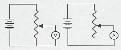
The temperature coefficient of resistance can be investigated with a copper wire wound resistor and a carbon resistor. A small circuit with a battery, lightbulb and resistor is set up and then the resistor is put into a cup of liquid nitrogen. The change in light brightness indicates the sign of the temperature dependence. The temperature dependence of a semiconductor can be investigated by dipping a large green LED into liquid nitrogen and noting the color change.
Because any battery has an internal resistance ri its terminal voltage VT drops when current is drawn from it;
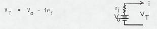
whereVo is the open circuit voltage. Measurements of VT for various i's are taken so ri can be determined. The circuit and operation are described over.
Students will be familiar with this effect from trying to start a automobile with the lights on. When the starter motor is actuated, the lights become noticably dimmer as the terminal voltage of the battery drops. A 12 V light bulb is provided in this circuit so the class can see it get dimmer as the large currents are drawn.
As of September 1979, the internal resistance of The J.C. Penney Battery was 0.02 ohms so it could deliver 600 A to a short circuit.
The circuit board for this demonstration allows the control and measurement of large currents (100 A) from a storage battery. The large currents are also used for magnetic fields of currents demonstrations.
High-Current Control Circuit
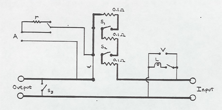
Basically the circuit routes the current from a 12 V storage battery through a series of 0.1W power resistors. When S2 is in the left position, the current passes through only one resistor, and will reach 120 A if there is no other resistance in the circuit. The single power resistor will heat up rapidly so this position must be used only momentarily. When S2 is in the right position, the current passes through the second power resistor. With S1 in the left position about 60 A will flow to a closed circuit; with S1 in the right position, the current flows through the third power resistor and 40 A flows.
The switch S3 is provided to short circuit the output for terminal voltage and internal resistance measurements.
The shunt w adjusts the Leybold 60 mV/300 mA meter to read 100A full scale at A, or 333 A full scale on its red scale when the series resistance r is switched in.
A voltmeter is hooked to V to read the terminal voltage of the battery.
Several multirange meters for measuring voltage and current in AC or DC are available including two large Leybold meters that can be used to monitor voltage and current in a circuit, and a large display digital multimeter that will measure voltage, current, resistance, and temperature.
Some professors have used the digital ohmmeter as a "lie-detector" -- a student volunteer was called up to answer embarrassing questions while holding the leads of the ohmmeter.
There are also large standing galvanometers, a model of a meter movement, and a measuring amplifier reading out onto a large meter for measuring small currents of 10-7 to 10-11 amps.
A person pushes the pedals of the the bicycle to generate enough current to light up to eight parallel light bulbs. The more bulbs the more resistance. Try it. you'll see.
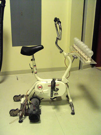
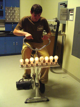
Two solenoid coils connected by wires are arranged so that magnets on springs oscillate in them. When one magnet is set oscillating, the induced current causes the other to oscillate also.
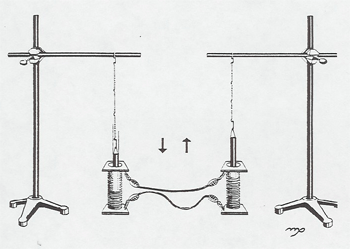
In a variation of this demonstration known as Nefkens's Telephone the two coils are set on opposite sides of the lecture hall with a long wire connecting them. Just by arranging some pieces of iron and copper in the right way, movement here causes movement over there -- an astonishing achievement of the mind of Man.
Short the leads of one of the coils and the oscillation of the magnets will be rapidly damped out by Lenz's Law.
This apparatus is used in an 8E lab experiment. A spherical electron tube is mounted inside of a Helmholtz coil setup. The electrons are projected to circle in the magnetic field, and you measure the radius of the circle, the current to the Helmholtz coils, and the accelerating voltage to determine e/m. The electron path is made visible by dim ionization of the residual gas in the tube.
If the tube is twisted a little inside the coils, the circle becomes a helix. This is a very pretty demonstration of the path of charged particles in a magnetic field.
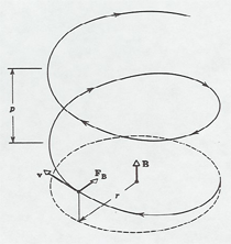
- The following experiments may fatally damage your microwave and will probably start a fire in your kitchen.
- A microwave oven can be used for various demonstrations including standing waves in an overmoded wave guide cavity, heating by electromagnetic waves, creation of plasma balls fed by microwaves, conduction of hot glass, superheating of fluids and others. A neon tube array shows the electric field pattern. Click on the picture of the array below to see a video of the array in the oven.
E-field in Microwave Oven
Lightbulbs in a Microwave Oven
Microwave Plasma Balls
A magnet thrust into a coil produces a noticable deviation on a table galvanometer. Or the coil can be moved over the magnet. (See also Special Relativity Demonstration [70])
In another demonstration two large coils are placed adjacent to each other, one connected to the galvanometer. When the other is pulsed with a battery, the induced current will be noted on the meter. You can emphasize the point that a steady current in the primary will induce no current in the secondary. If an iron core is positioned through the two coils, the galvanometer readings will become dramatically larger.

Faraday Bulb
A coil connected to a small bulb is mounted on a disk. When the disk spins the coil through the poles of a magnet, the bulb lights for that part of the arc for which the coil is passing through the magnet.
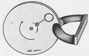
A small vacuum tube transmitter feeds an electric dipole antenna. The EM waves with l = 3m are picked up by a handheld dipole receiving antenna and detected by a peanut light bulb. Several aspects of dipole radiation can be illustrated with this setup:
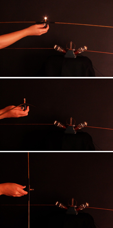
Modern Version of Hertz Wave Experiment
A VCR is set up with a videotape broadcasting on Ch 3. Instead of wiring the cable directly to the TV, it goes instead to a folded dipole antenna optimized for the frequency of Ch 3, which is 60 66 MHz. The receiver is a second folded dipole antenna which is connected to the TV (tuned to Ch 3), which acts as the detector.
It is easy to diplay the polarization of the EM waves by turning one of the dipole antennas at a right angle to the other. If there are standing waves in the room these can be seen by moving one antenna in relation to the other. From the distance between nodes the wavelength can be determined.
TV stations have a 6 MHz bandwidth. Channel 3 is 60 66 MHz which gives a wavelength of 5 meters. How are TV antenna oriented on a roof? That gives the polarization.
FM frequencies are 88 108 MHz
Broadcast antenna are horizontal or 45o
AM 550 1600 kHz
Vertically polarized antenna, usually center-fed dipole with image in ground.
Cellular phone antenna usually have a 10-60cm wavelength. From the antenna size you can guess the frequency.
The antenna used in this demo are folded dipole type made from 300 Ohm twin lead. They are connected to 75 Ohm cable through impedance transformers.
To see how the radio spectrum is divided up by users press here. [71]
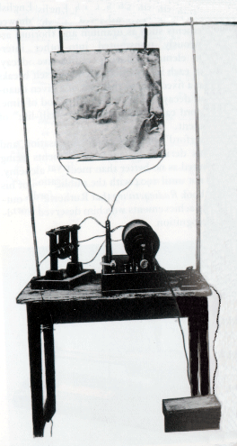
A radio transmitting apparatus used by Marconi in 1895 in some of his earliest experiments.
You can show the rainbow spectrum of visible light with a dispersing prism [73] in front of a slide projector. A transparency of Maxwell's Rainbow, next page, is available.
An infrared detector connected to a meter visible to the class is placed beyond the red in the spectrum above. Why is the signal so small? Doesn't the tungsten lamp peak in the infrared? Ah, remove the "heat" absorbing glass element from the projector and the signal becomes large.
Ultraviolet light and the fact that it is absorbed by window glass can be demonstrated in connection with the photoelectric effect [74].
A radiometer consists of a spinner in a near vacuum with vanes silvered on one side and blackened on the other. When light, particularly infrared, falls on the radiometer, the black sides of the vanes become hotter and drive residual air molecules away from them, propelling the vanes around. (The rotation direction is contrary to that produced by radiation pressure, a smaller force.) A flashlight will operate the radiometer, but a match flame, which has more infrared, does much better. (Low powered lasers, of course, have too little energy to operate the radiometer.) Parabolic reflectors can be used to focus the infrared from a match or electric coil to spin the radiometer across the lecture hall.
Jumping Ring
A light aluminum ring, when placed on the iron core sticking out of a large AC electromagnet, is ejected violently into the air when the electro-magnet is activated. The conceptual explanation is that the AC magnet is continually reversing polarity, and induces a voltage in the ring so the ring's magnetic field continually opposes (repels) that of the iron core.
Copper rings and split rings are available to test also. A heavier copper ring will float midway up the iron core. When the ring is forced down on the iron core, it becomes very hot. A split ring will not move; it is not a complete circuit.
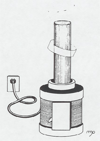
Magnetically Damped Pendulum
A pendulum with various disk is arranged to swing through the poles of a powerful permanent magnet. A solid aluminum disk is stopped on the first pass. An aluminum disk slotted to reduce eddy currents is moderately damped, and a cardboard disk swings freely.
Various rectangular plates can be released to fall through the poles of the magnet. An aluminum plate slides viscously, a slotted plate more rapidly, and a cardboard plate is unaffected.
Russian Version
Two rings are balanced on an arm which swings freely on a bearing. When a magnet is thrust into one ring, it is repelled away. (You can use this to illustrate the answer to the question in connection with the Faraday demonstration [75], "Where does the energy come from that moves the galvanometer needle?"). When the magnet is pulled out, the ring is attracted towards it. The other ring is split; thrusting a magnet in and out has no effect on it.
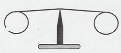
Osheroff Demonstration
A copper plate is cooled with liquid nitrogen to improve its conductivity. A falling magnet bounces without hitting the plate and lands on it's edge.
A large DC motor, with easily visible coils and split-ring commutator, operates from a 6 V battery. The motor can be rewired so that the field coils are energized. If the armature is now rotated by hand, a DC current is generated.
An AC-DC motor-generator has a single turn armature and both split and slip rings to act as a DC motor or an AC or DC motor or generator.
A hand-crank generator illuminates a neon bulb when cranked vigorously.
A small coil, mounted near the edge of a plexiglass disc, is connected to a peanut bulb. When the disc is spun between the poles of a powerful permanent magnet, the bulb is seen to be lit for that part of the circumference for which the coil passes through the poles of the electromagnet.
A tin can induction motor is demonstrated by holding a tin can on a special handle near two large coils at right angles. The coils are connected to the AC line, but one has a series capacitor to shift its phase 90° with respect to the other. This illustrates the starting circuit of the most common type of electric motor, the induction motor.
The hand-cranked generator is wired through a knife switch to an incandescent bulb. You can use a student volunteer to verify that it is much harder to crank the generator when the bulb is in the circuit, than when no current is being drawn. Ask your class why.
The Magnetic Levitator [76] has two coils at right angles connected to 120 VAC so the coils are 90° out of phase. These will rotate the suspended ball as in the tin can motor.
The secondary of a 1:1 transformer is hooked through a switch to a light bulb. The primary is hooked in series with another light bulb to the 120 V. line. When the switch is open neither bulb lights; the inductive reactance of the primary keeps the current small in the primary circuit. But when the switch is closed, both bulbs light! Now the secondary circuit is drawing current, so the mutual inductance of the two coils reduces the effective inductive reactance of the primary and enough current flows in the primary circuit to light its bulb.
Alternatively, conservation of energy tells us that the primary current must increase so that energy can be delivered to the secondary bulb through the magnetic fields linking the coils.
![]()
The Paul Trap, or rotating saddle trap, is an analogy to RF-electric quadrupole ion traping.
A Tesla coil is a high frequency, very high voltage transformer. The operation and circuit are described below. Our smaller Tesla coil radiates enough RF to illuminate a fluorescent tube a foot away. You can draw a one foot arc into your body, using a metal rod; the frequency is so high that the ions in your body do not have time to move far enough to do damage.
The Giant Tesla Coil generates a four foot discharge that will illuminate fluorescent tubes many feet away, and will generally terrify anyone anywhere near it. People with pace makers are supposed to move to the back of the room.
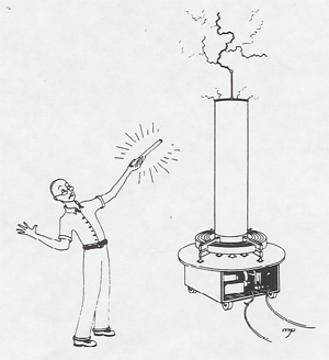
Tesla Circuit Operation
A preliminary step-up transformer boosts the line voltage to ten or twenty thousand volts. (A neon sign transformer is used for this purpose in the giant Tesla coil.) This voltage arcs across the spark gap F at 60 Hz, ringing the tuned circuit consisting of the capacitor C and the Tesla primary (a few turns) at 1-3 MHz. The Tesla secondary (many fine turns) has its own resonant frequency determined by its inductance and the internally distributed capacitance between its windings. The primary LC circuit is tuned to this resonant frequency for maximum coupling.
A spectacular demonstration with the small Tesla coil is to hold a fluorescent bulb in one hand and a metal rod in the other. When you draw an arc with the metal rod from the Tesla coil, the current passes through your body and lights the bulb. The voltage is over 1 million volts; why doesn't it shock or kill you? There are a number of hypotheses on this: a. The skin effect -- the current travels in the outer dead layer of skin. b. Human nerve circuits do not respond to high frequencies like 1 MHz, perhaps because of the reason mentioned above; there isn't time for the sodium and potassium ions to move far in the nerve cells. c. The impedance of the Tesla coil is very high, and it therefore induces only very small currents in humans.
A skin depth calculation using the conductivity of sea water, sigma = 4 mhos/m, gives a depth of 0.25cm, so this effect would not play a large role in protecting you, at least from pain stimulation on the skin surface. The answer is probably a combination of effects b and c from above. The current through the body is too small to generate enough heat to injure the person, and the high frequency does not stimulate pain nerves, or induce muscle contraction.
Our giant Tesla coil does sting you if you get into its circuit path to the ground. Tesla coil builders claim that the "gentleness" of the particular Tesla coil depends on the cleanness of the separation of 60 Hz and the high frequency at the spark gap.
A nice description of how the tesla coil circuit really works is here [77].
A demonstration transformer steps the 110 V AC line voltage up to 10,000 V for a Jacob's Ladder. The current arcs across the shortest distance between two upright conductors. Once started the arc rises, owing to the heated air, and jumps over a distance of several inches.
A secondary of few turns can be substituted to make a stepdown transformer. The low voltage - high current can be used to spot weld sheet metal or to melt a tin ring.
Transmission Line
![]()
A signal generator capable of 10 MHz is hooked to a T-connector at channel 2 of an oscilloscope through an 8 meter 50 ohm cable as shown above. Channel 1 of the scope is hooked to the same source through a short cable.
Input a pulse at 1 MHz; sweep at 0.5 ms/cm
Input a sine wave
Suggested by Brad Tippens
In the ideal case the magnetic field lines of a toroidal coil are entirely contained witnin tne coil and = 0 outside. This can be checked by using a flip-coil, Hall probe, or compass needle near the toroidal coil.
However, the lines of vector potential circle the flux lines:
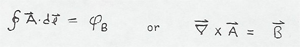
So A is not zero outside the coil.
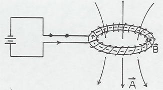
If a wire is threaded through the hole of the toroid and returned through the hole, case 1, no galvanometer deflection is seen as B is switched on and off. But if the wire is threaded through the hole and returned around the coil, case 2, a galvanometer deflection will be seen from = -d/dt.
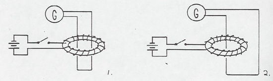
Protoboards, 15V and other power supplies, meters, components, etc. are available for hooking up your own electronic circuits.
A small solar cell when placed under a flood light runs a propeller.
The intrepid researchers in the demolab have discovered the secret of Blue Love. It's electricity. One side charges up positive, and one side negative. See for yourself.
The apparatus is shown below.
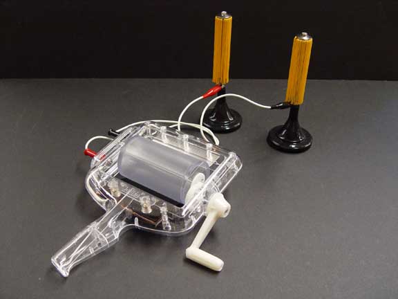
This is a very nice demonstration of Coulomb's Law with a fancy torsion balance and Laser spot readout. You can show that the electrostatic force varies as the square of the distance and is proportional to one of the charges. It is probably a good idea to practice a little with this one before hand.
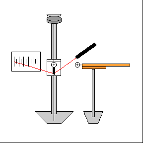
This is a very impressive demonstration which will draw lots of comment! It can be used to emphasize the difference between conductors and insulators.
The dissectable Leyden jar is charged up with a Van de Graaff and then discharged by shorting the inner and outer can to show charge storage. Then the jar is recharged and disconnected from the Van de Graaff. The inner can is lifted out with an insulated tool, or, with care, by hand. At this point the parts of the jar are safe to handle, and the glass jar can be lifted out, the inner and outer cans touched to each other, or touched to the glass jar in any combination. You can even give the pieces to the students to handle.
When the Leyden jar is reassembled, the last step of inserting the inner can being done carefully, it will be found that the jar is still charged, as can be checked by shorting its terminals and drawing a spark.
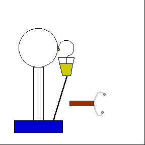 |
 |
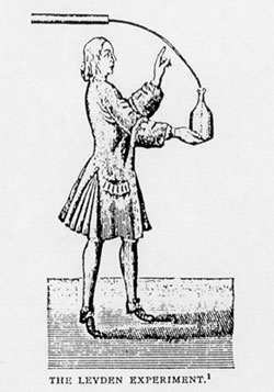 The discovery of the Leyden jar as described in a letter written by Musschenbroeck to Reaumur in 1746.
"I wish to inform you of a new, but terrible experiment, which I advise you on no account personally to attempt. I am engaged in a research to determine the strength of electricity. With this object I had suspended by two blue silk threads, a gun barrel, which received electricity by communication from a glass globe which was turned rapidly on its axis by one operator, while another pressed his hands against it. From the opposite end of the gun barrel hung a brass wire, the end of which entered a glass jar, which was partly full of water. This jar I held in my right hand, while with my left I attempted to draw sparks from the gun barrel. Suddenly I received in my right hand a shock of such violence that my whole body was shaken as by a lightning stroke. The vessel, although of glass, was not broken, nor was the hand displaced by commotion: but the arm and body were affected in a manner more terrible than I can express. In a word, I believed that I was done for."
An E-field projection device with self-contained fluid is available. You can change the electrodes and show several different field patterns such as +/- point charges, parallel plates and others in a few minutes. This device is charged by a piezoelectric gun, not the Van de Graaff as shown in the animation below.
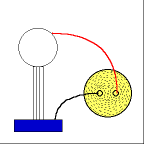
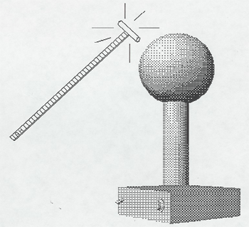
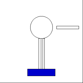
The equipotentials of a charged sphere are concentric spheres centered on the charged sphere. A small fluorescent tube is held on a plastic meter stick near the charged Van der Graaff sphere. When the tube is along a radial line of the sphere, the tube lights; the ends are at different potentials. But when the fluorescent tube is held tangent to a concentric sphere, the tube does not light; the ends are at the same potential.
To show that work is done in bringing a charge up close to another charge, alternately touch the grounded discharge rod to the Van der Graaff sphere and move it away. When the sphere is grounded the motor driving the belt runs faster - -more freely. No work is done to bring charge up. But when the grounding rod is moved away, the motor slows down, "lugging" away to carry charge up the belt close to the charge building up on the sphere. The charge carried up on the belt is delivered to the center of the sphere, whence it quickly moves to the outside of the sphere in obedience to Gauss's Law. As the charge on the sphere builds up, it begins to leak into the air. Equilibrium is reached when the charge leaks off the sphere as fast as the belt is able to bring new charge up.
An electrophorus consists of a flat insulator on which rests a removeable metal plate. The Lucite base of the electrophorus is charged positive by rubbing it with silk. When the metal plate is placed on it, the metal contacts the lucite in only a few spots and acquires very little positive charge. But if the metal plate is now grounded (by touching it with your finger), it acquires a large negative charge by induction.
The metal plate is now lifted off and its negative charge can be detected at some distance with an electroscope or with pith balls. The charged plate will cause a half-inch spark to jump to your knuckles (painless), or it will flash a neon or fluorescent tube briefly (best seen by turning off all lights).
The operation of charging the metal plate by induction can be repeated indefinitely, since essentially no positive charge is removed from the insulator base. You may wish to ask your class where the energy comes from, which could be used to flash a fluorescent tube indefinitely.
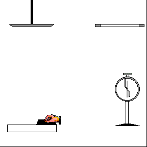
This demonstration uses a Van der Graaff generator, a 10 cm test sphere on an insulating handle, a can mounted on an electroscope (the "ice pail"), and a second electroscope to test for charge. The "medium" difficulty of the demonstration is in remembering to do all the steps in the correct order.
Version 1: The induced charge equals the inducing charge

Charge the small sphere with the Van der Graaff. Ground the Van der Graaff sphere and the pail to make sure there is no extra charge around. Show that the small sphere is still charged by bringing it near the second electroscope.
Lower the small sphere into the pail without touching it. The electroscope deflects. Remove the sphere, and the deflection disappears.
Lower the sphere into the pail again without touching it. The electroscope deflects. Ground the pail by touching it. The deflection disappears. Remove the sphere. The electroscope deflects again. You have induced a charge, opposite in sign to that on the sphere, onto the pail from the ground. We will now prove that the magnitude of this induced charge on the pail is equal to the magnitude of the charge on the sphere.
Lower the sphere slowly into the pail. The deflection goes to zero. Lower the sphere down until it touches the bottom of the pail. If you listen carefully, you can hear the sound of the spark jumping. The deflection remains zero. Now take the sphere out. The deflection remains zero, and you can test the there is no charge on the sphere by bring it to the second electroscope. All charge has been neutralized.
Suggested by Bill Layton
Version 2: Gauss's Law
Start as above. Charge the small sphere and lower it into the pail without touching it. The electroscope deflects. Remove sphere. Deflection disappears. Put sphere back in. Deflection returns. Lower the sphere so it touches the bottom of the pail, and you can hear a spark jump. Deflection remains unchanged. Remove the sphere. Deflection remains unchanged. Finally, bring the sphere to the second electroscope. There is no deflection. The sphere is completely discharged. All of the original charge on the sphere went over to the pail.
When a charged cloud went overhead the bells rang to alert Franklin so that he could do his experiments. A pair of pith balls allowed him to determine which charge (positive or negative) the cloud carried. We have a set of Franklin's bells that can be charged with the Van De Graaff Generator.
That charge is only on the outside surface of a conductor is shown by several demonstrations.
| a. A hollow cylinder is connected to a Van De Graaff generator. Pith balls hanging on the outside fly up wildly but pith balls hanging from the inside barely stir. |
|
|
b. Faraday Cage - -When a Van de Graaff is turned on, it will affect an electroscope at a distance of a meter or more. However, when a metal cage is put over the electroscope, the electroscope is not affected, even if the apparatus is moved close enough so sparks jump to the cage. |
|
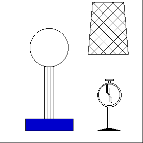 |
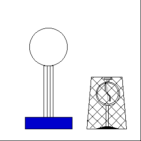 |
| c. Faraday Pail - -a small metal can is placed on the electroscope. A "charge carrier" (a small metal ball on an insulated rod) is used to transfer charge from an electrophorus plate or Van de Graaff sphere to the inside of the can. Since this charge immediately flows to the outside of the can, several more "spoonfuls" of charge can be added to the can in this manner, as shown by the increasing deviation of the electroscope leaves or needle. This, then, is the principle of the Van de Graaff generator - - charge is continually carried up by the belt to the center of the sphere, whence it accumulates on the outside. |
|
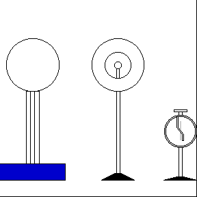 |
d. A very definitive demonstration of Gauss's Law is provided by a large hollow sphere with an opening in the side and an electrode in the center. The hollow sphere is charged by connecting a conducting rod from the center electrode to a Van de Graaff generator. Charge can now be removed from the outside of the hollow sphere by touching it with a charge carrier. The charge carrier is touched to an electroscope to show the presence of charge. But if the charge carrier is touched to the center electrode of the charged hollow sphere, no charge can be removed. All the charge has flowed to the outside of the sphere. (The insulated metal ball of the charge carrier should be touched very gently to the electroscope; otherwise, the indicating needle will be banged up, confusing the students.) |
Cold, dry days are best for these demos.
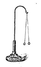
| a. A rubber rod is charged negative by rubbing it with rabbit's fur. A lucite rod is charged positive by rubbing it with silk. When one charged rubber rod is placed in a stirrup, another charged rubber rod will repel it, but a charged Lucite rod will attract it. This simple but graphic demonstration shows that charges come in two sorts. | |
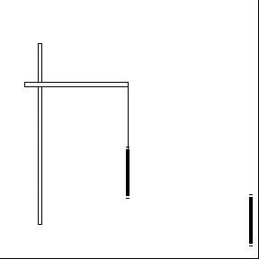 |
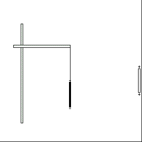 |
 |
b. The charged rods will pick up bits of paper and styrofoam by polarization. |
| c. The charged rods will first attract hanging pith balls by polarization. When the balls touch the rod, they acquire some of its charge and thereafter are repelled from the rod strongly. The pith balls now hang apart, repelling each other. | 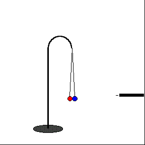 |
 |
d. If a charged rod is brought near an electroscope, its leaves will diverge. If the rod is touched to the electroscope, the leaves will remain diverged, even when the rod is moved away. The electroscope can be charged by induction by grounding it with your finger when the charged rod is near. Remove your finger and then the rod, and the electroscope is now charged with the opposite charge of the rod. This can be checked by bringing the charged rod near again; the leaves now come together. |
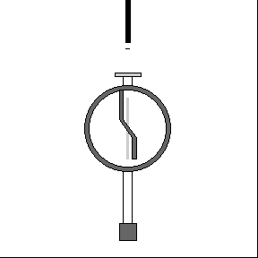 |
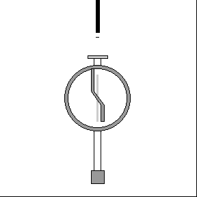 |
Note: All electrostatic demos work better on cold, dry days.
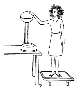

| a. Charge flows to the points and sprays off. In this classic demonstration, the professor or a student volunteer stands on the insulated base and places his/her hand on the sphere of the generator. An assistant turns the generator on, and the demonstrator's hair stands on end. The demonstrator should have a key or other pointed object concealed on his person to hold up and spray off the excess charge when the demonstration is over.
A similar effect can by demonstrated by placing a wig on the sphere, or by connecting the sphere to a paper plume. The electric flier shown below will spin by spraying off charge when connected to the sphere. |
|
 |
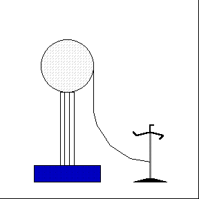 |
| b. Action of a lightning rod. Two Van de Graaffs are provided, one of which charges its sphere positive, and the other negative. When both are turned on, they will spark to each other over 8 -12" distance. However, if a small point is placed on one sphere, aimed in any direction, even at the other sphere, no sparks will jump, because the point dissipates the charge into the air preventing the potential from building up. | |
 |
 |
| c. Charge density is Greatest at the areas of highest curvature. When the pear-shaped metal sphere is charged by touching it to the Van de Graaff, a larger charge can be removed from the narrow end than from the fat end. The amount of charge is tested by the deflection of an electroscope. To produce a noticeable effect this demonstration must be done carefully. | 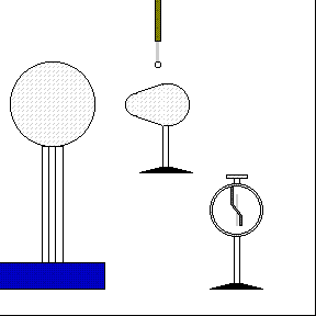 |
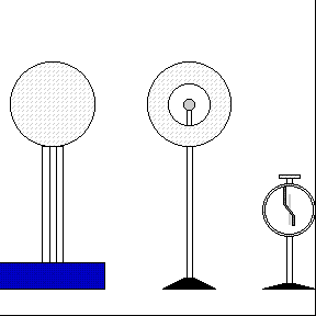 |
d. Gauss' Law --charge is on the outside of a conductor. Several demonstrations of these effects are described here [78]. |
| e. Conductors and non-conductors. A string connected between an electrostatic generator and an electroscope will not conduct charge, but a metal wire will. | |
 |
 |
| f. Smoke precipitator. Smoke blown into a tube (from a cigarette) rapidly disappears when the electrodes on the ends of the tube are connected to the generator. |  |
|
|
g. "Shot from guns" A paper cup full of puffed wheat or small Styrofoam chips placed on top of the generator produces a spectacular effect. Bring your own puffed wheat. |
The Wimshurst Static Machine generates large sparks for entertainment or for use in various electrostatic experiments. The associated Leyden jars can be connected in or out of the circuit to illustrate the function of a capacitor -- in circuit, the sparks are much fatter and louder (Q larger), but of the same length (same maximum V), and much less frequent (longer time to build up the large Q).
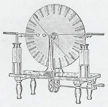
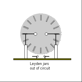 |
 |
In 1994 Andrew Alcon patented* a simple device which stably levitates a magnet above two counter-rotating aluminum rotors.
The motors used in this demo are 5,000 RPM, 1/15 HP, 115 VAC Dayton model 2M066. The aluminum rotors are carefully made to spin true. A light dimmer circuit is used to control the speed of the motors.
*US Patent 5,319,336
The small floating magnet is balanced against gravity by the upper ring magnet. This levitation configuration is unstable vertically, but stability is provided by the diamagnetic carbon plates above and below the floating magnet. The diamagnetic material produces repelling forces as the floater approaches, pushing it back to its center position and overcoming the vertical instability.
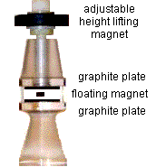
A small sample of a type I superconductor will demonstrate the Meissner Effect (levitating a magnet) when cooled in liquid nitrogen.
Another example of superconductivity can be demonstrated using a type II superconductor.
A piece of superconducting material is cooled with liquid nitrogen on top of a track array of magnets. When the superconductor cools, it floats atop the magnetic array. If the track is turned upside down, the superconductor goes from being levitated to suspended due to flux pinning which freezes the magnetic flux within the type II superconductor.
Video of diamagnetic levitators showing many objects including hazelnuts, strawberries, and a living frog.
An electromagnet suspends an iron ball in mid air. An IR LED and phototransistor pickup senses the position of the ball, and the associated electronic circuitry controls the current to the magnet by active feedback. Two other magnets 90° apart and 90° out of phase can cause the suspended ball to spin.
A wire in the form of a trapeze swing hangs between the poles of a powerful magnet. When a current is passed through the wire, it jumps violently out from the poles.
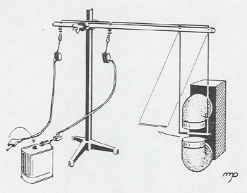
A power resistor set-up is used with a storage battery to deliver a hundred amperes to a heavy copper wire to orient iron filings or compass needles for overhead projection.
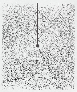
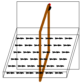
This demonstration is an excellent illustration of tne vector cross product. A beam of electrons is outlined on a fluorescent card in the tube. A magnet brought near the beam neither attracts it or repels it, but bends it "sideways" according to the F = qv x B law.
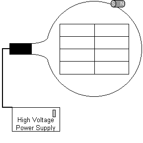 |
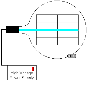 |
A magnet deflects the large curly filament of a light bulb connected to a DC source. If an AC source is used, the filament vibrates impressively (See AC-DC Difference [80]).
A model of a meter movement shows how a coil rotates in the field of a permanent magnet when a current is pulsed through it.
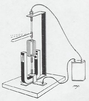
Often during his lectures at the University of Copenhagen H. C. Oersted had demonstrated the non-existence of a connection between electricity and magnetism. He would place a compass needle near to and at right angles to a current carrying wire to show that there was no effect of one on the other. After one of the lectures a student asked, "but, Professor Oersted, what would happen if the compass needle was placed parallel to the current carrying wire?" Oersted said, "Well, let's see," and went down in the history of physics; the student's name is forgotten.
(Adapted from H.E. White, Modern College Physics, pp 433, D. Van Nostrand, Princeton, 1962)
Large currents passed through two neighboring parallel wires cause them to attract dramatically, or to repel if the currents are passed antiparallel.
A box with parallel and antiparallel wires made of aluminum foil exists for lecture demonstrations. The box sits on the overhead projector and is powered with a 12V supply. The motion of the wires is easily detected by the class as the experiment is magnified on a screen.
A long straight wire demonstration, a solenoid field, and a field of a current loop are available in compass table form. Many tiny compass needles turn to outline the magnetic fields for overhead projection, saving you the trouble of carefully spreading the iron filings.
A similar arrangement for overhead projection shows the magnetic field of a loosely wound solenoid coil.
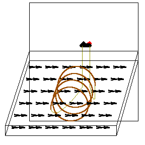 |
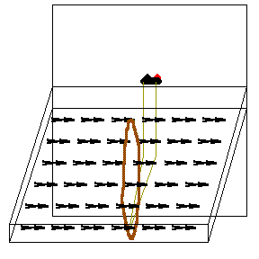 |
Domains are well modeled by the compass table, an array of about one hundred small compass needles used for showing fields of bar magnets, etc. When there is no strong external B-field, sections of the array line up in different directions, each individual compass needle aligning itself with the local field. When the array is tapped sharply, it will be seen that the needles on the boundaries of the domains are the least stable (vibrate the most), and some of them realign causing one domain to grow at the expense of another.
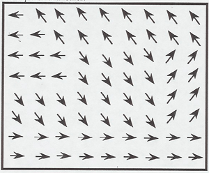
In the Barkhausen effect, a large coil of fine wire is connected through an amplifier to a speaker. When an iron rod is placed within the coil and stroked with a magnet, an audible roaring sound will be produced from the sudden realignments of the magnetic domains within the rod. A copper rod, on the other hand, produces no effect.
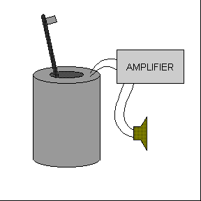
This pretty demo uses a "permalloy" rod, a soft iron rod, a hammer, and the compass dip needle (which is shown here [81]).
|
|
Using the dip needle find the direction of the earth's magnetic field in the class room (plunging about 60° earthward to the magnetic north). Arrange the soft iron rod perpendicular to the earth's field, and strike its end several times with a hammer. This insures that it is demagnetized, which is demonstrated by showing that either end of the rod will attract either end of the compass needle (by magnetic polarization). Now align the rod with the earth's field and strike it several times to shake its domains around and magnetize it. That the rod is magnetized is demonstrated by showing that the north end of the rod repels the north end of the compass needle and the south end of the rod repels the south end of the compass needle. This rod retains its magnetization, no matter how it is oriented in the earth's field.
However, the permalloy rod is so compliant that if held along the earth's field its north end will repel the north end of the compass needle, and now if it is smoothly reversed without any hammer strikes, the other end will repel the north end of the compass needle! Its domains line up with the earth's field without any impact blows.
A small wheel has monel metal wrapped around its circumference. A small light bulb is positioned to heat one part of the circumference, raising the metal above its Curie temperature so it no longer responds to magnetism. When the wheel is placed in the field of a strong magnet, it rotates slowly as one part of the circumference is continually rendered non-magnetic by the heat of the light bulb.
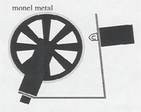
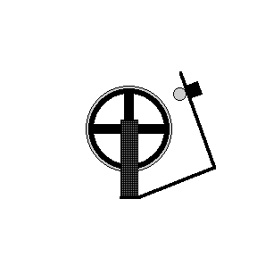
A nickel paper clip (a regular steel one is available too) attached to a base with a string is suspended in air by the use of a magnet. If the nickel paper clip is heated with a lighter (for the steel paper clip a blowtorch is required) beyond a certain temperature called the Curie temperatures it is no longer attracted by the magnet.
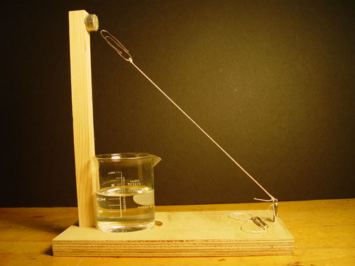
The Curie temperature (Tc) is the critical temperature beyond which a previously ferromagnetic material becomes paramagnetic. On the atomic level, below the Curie temperature the magnetic moments, contributed mainly by the electrons, are aligned in their respective domains and even a weak external field results in a net magnetization. As the temperature increases to Tc and above however, fluctuations due to the increase in thermal energy destroy that alignment. Tc for nickel is 631K, while that for iron is 1043K.
A magnetic declination and inclination needle is provided for determining the direction (deviation and dip angle) of the earth's magnetic field in the classroom.
A globe of the earth may help to illustrate these concepts.
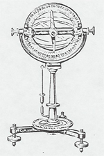
The total magnitude of the magnetic field vector is about 0.5 Gauss units or equivalently 50,000 nanoTeslas (nT). To find the components of the magnetic field anywhere visit the Standard magnetic Field Model [82] and enter the date, and your geographic latitude, longitude and elevation. The table below shows the representative components for June 1, 1999 at sea level. Bx, By and Bz are the components in units of nT, B is the total field strength also in units of nT, D is the declination angle between geographic and magnetic north, and I is the inclination or Dip Angle, in degrees below the local horizontal plane.
Average Magnetic Components
| City | Bx | By | Bz | B | D | I |
| Los Angeles | 24276 | 5996 | 41636 | 48568 | 13.9 | 59.0 |
| New York | 19308 | -4643 | 50289 | 54068 | -13.5 | 68.5 |
| Boston | 18006 | -1566 | 53490 | 56461 | -4.9 | 71.3 |
| Chicago | 18686 | -803 | 52908 | 56117 | -2.5 | 70.5 |
| Miami | 25478 | -2182 | 38586 | 46290 | -4.9 | |
| Huston | 24892 | 2050 | 42441 | 49245 | 4.7 | 59.5 |
| Denver | 20895 | 3878 | 49938 | 54272 | 10.5 | 66.9 |
| San Francisco | 23004 | 6411 | 43851 | 49932 | 15.5 | 61.4 |
There are 3 ball bearings stuck to a magnet in a track. A fourth ball bearing is released on the opposite side of the magnet, and is attracted to it. The ball at the other end shoots off at a much higher velocity. Where does the energy come from?
A second version of the gauss cannon is below and uses one spherical magnet which looks identical to the ball bearings. The device can first be shown without the magnet, when it acts like Newton's cradle and conserves energy. With the magnet, the end ball shoots off the end of the ramp.
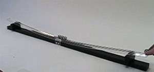
The circuit below, from Physics Demonstration Experiments Volume 2 by Harry Meiners, page 972, will draw a hysteresis curve on the oscilloscope. The twenty ohm resistor serves to measure the current to the transformer primary producing a horizontal signal proportional to H. The output of the secondary of the transformer is proportional to dB/dt. The final RC circuit integrates this (see RC Integration and Differentiation [83]) to produce a vertical signal proportional to B. As you adjust the variac to control the current to the primary, the curve on the oscilloscope stretches out to saturation.
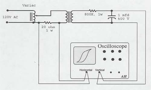

A compass table with a hundred or so tiny compass needles displays the magnetic field of a bar magnet, or two attracting or repeling magnets, for overhead projection. The compass table replaces the old iron filing magnetic field demonstrations (which are still available).
 |
 |
Compass tables are also used to show the magnetic fields of a long straight wire, a solenoid coil, and a current loop (see Solenoid and Loop Fields [84] and Parallel Wires [85]). The "magniprobe" is a tiny bar magnet completely free to rotate on gimbals in any direction. It will display the three dimensional form of the magnetic field of a bar magnet, delighting the instructor. However, the device is too small to be seen by more than a few students at once unless enlarged on TV. The "Mark II" version of the magniprobe is sensitive enough to detect the earth's field.
| Various magnets and compasses are available; the strongest magnets are the little ceramic magnets, these can be handed around to the class. |
|
| A piece of lodestone picks up small iron objects, or can be suspended so as to point north. | |
 |
 |
| A large, strong bar magnet repels another held by braces and suspends it several inches in the air. |
|
| Using the dip needle find the direction of the earth's magnetic field in the class room (plunging about 60° earthward to the magnetic north). Arrange the soft iron rod perpendicular to the earth's field, and strike its end several times with a hammer. This insures that it is demagnetized, which is demonstrated by showing that either end of the rod will attract either end of the compass needle (by magnetic polarization). Now align the rod with the earth's field and strike it several times to shake its domains around and magnetize it. That the rod is magnetized is demonstrated by showing that the north end of the rod repels the north end of the compass needle and the south end of the rod attracts it. | |
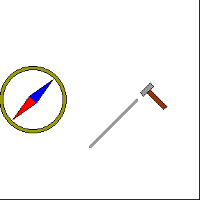 |
|
| A small electromagnet operated from a battery will pick up nails, etc. |
|
|
|
A giant compass needle is useful for demonstrating the earth's magnetic field and for determining the north and south poles of various magnets. |
A torsional balance contains various vials of paramagnetic and diamagnetic material including graphite and gadoliminium oxide.
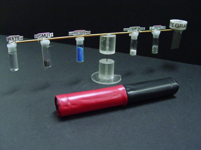
![]()
Diamagnetic graphite can be used to stabilize magnetic levitation.
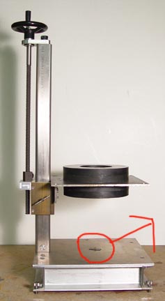
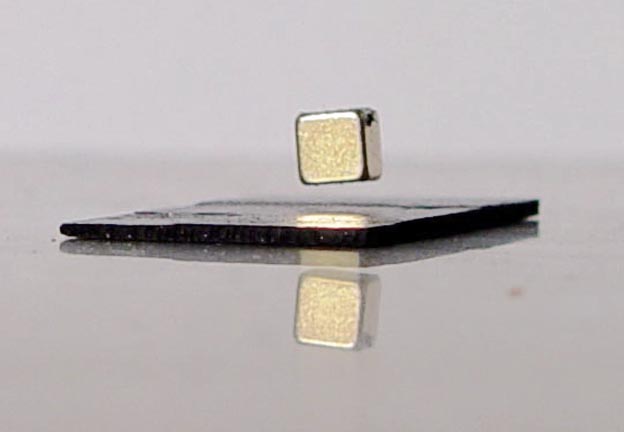
![]()
Microscopic graphite dust is made of flakes which lie flat and reflect a silver light (left view). When put over a magnetic field, the flakes stand up on edge due to graphite's diamagnetic property (right view). Only the top edges reflect light, and the powder looks very black. Light goes in, scatters into the deep valleys, and never comes out. The blackest black has been produced using a forest of aligned carbon nanotubes.
Rowland's Ring is used to demonstrate the magnetization curve of iron. (See Halliday and Resnick, Part II, Sec. 37.6) We have an actual Ring, or the Leybold demountable transformer will serve.
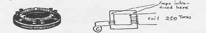
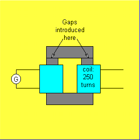
The flux in the iron is measured by switching off the current in the energizing coil and recording the reading of a ballistic galvanometer hooked to a pickup coil. (You can show that the maximum reading of a ballistic gavanometer is proportional to q = i t, which is in turn proportional to the change in flux through the pickup coil. You can determine the constant of proportionality by discharging a known capacitor through the galvanometers.) The large demonstration galvanometer will serve as a ballistic galvanometer for lecture purposes.
Professor J. Oostens has suggested the following demonstration of magnetic saturation and reluctance:
The Leybold transformer is arranged as above. The experiment is run first with no gap for several values of the current. Then a small gap is provided with shims, and the measurements repeated for the same set of currents. A Hall probe and Gaussmeter can be introduced in the second case for more accurate measurements of B in the gap. Sample data are shown below:
| I
(amps) |
nI
(amp.turns) |
GFe
(units) |
GGap
(units) |
BCap
(Tesla) |
<--higher degree of accuracy. |
| 10 | 2500 | 1.2 | 1.3 | 0.89 |
Some deviation is due to a remiant field. (Iron behaves like a magnet for very low currents) |
| 5 | 1250 | 1.1 | 0.75 | 0.50 | |
| 3 | 750 | 0.95 | 0.45 | 0.28 | |
| 2 | 500 | 0.8 | 0.27 | 0.19 | |
| 1 | 250 | 0.7 | 0.1 | 0.090 | |
| 0.5 | 125 | 0.45 | 0.05 | 0.012 |
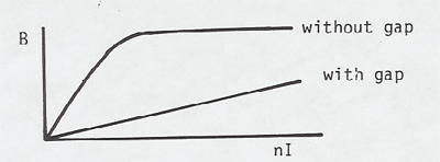
The graph shows that the field in the iron quickly reaches saturation. By computing the reluctance,
Reluctance = magnetomotive force / flux = nI / Φ
you can show that the reluctance of the air gap is much greater than that of the iron, even though the path length is much smaller.
An undamped compass needle vibrates about equilibrium in a B-field; the vibration frequency can be used as a measure of B. Let the (unknown) moment of inertia of the compass needle be I, and its (unknown) magnetic moment μ. Then the restoring torque τ=Bμsinθ. Using the analogy to linear harmonic motion the angular frequency of vibration is
ω = √ (k/m) = √ (Bμ/I)
Thus, the frequency of vibration of the needle is proportional to √B. Measure the frequency of vibration of the compass needle in the Earth's field of 0.5 gauss, and obtain the strength of other B-fields from these results.
Gauss Meter
Accurate and detailed measurements of B-field can be made with a Gaussmeter and Hall probe. You can illustrate the size of the gauss unit and the strength of various magnets, or make measurements of B-fields for electron deflection, etc.
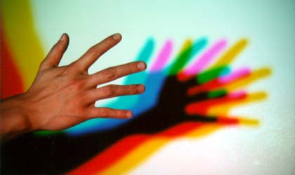
The kit has been improved with magnetic clamping to the blackboard and a multiple ray projector. Most of the principles of geometrical optics can be nicely demonstrated with this kit
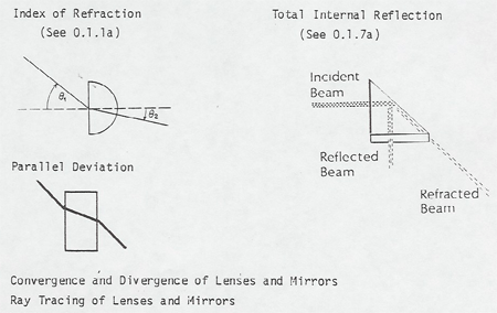
We have a light which magnetically clamps to the blackboard and projects five parallel rays. This dramatically shows convergence and divergence of rays in lenses and mirrors.
The Lenses and Mirrors applet below can be used as an online demonstration.
Physlet by Wolfgang Christian webPhysics, Davidson College [86]
Instructions on how to use the animation:
The setups below demonstrate the formation of the real, inverted image by a lens or mirror.
The laser is used in many demonstrations, but the students are delighted with the device itself.
First make a spot on the side wall and then catch it on your hand to show that the beam will not burn a hole through your hand. A short discussion of the dangers of looking down the beam is appropriate at this point.
Then place the laser on the table so the beam hits the side wall, walk along to the middle of the beam, and clap erasers over it so the pencil-like beam is outlined in falling chalk dust. We also have fog-in-a-can available for outlining the laser beam. (This is very effective.)
A similar stunning demonstration for a small group to gather around is to ask for a volunteer with a diamond ring. Beam the laser into the diamond, and clap chalk dust over it. The many tiny beams emerging from the diamond are very beautiful. The beam pattern can be used to "fingerprint" the diamond uniquely.
Another short demonstration is to place a human hair in the beam. From the resulting diffraction pattern and the wavelength of the laser, you can calculate the diameter of the hair.
A Metrologic publication "101 Ways to Use a Laser" is available.
A strongly converging lens shows obvious chromatic aberration. Another strongly converging lens is arranged so that the outer half of its diameter can be blocked (lens "stopped down"), or the inner half can be blocked (leaving an annular ring lens). The two arrangements have different focal lengths showing spherical aberration.
Other types of aberrations can be arranged with various lenses and mirrors.
The near (pn) and far (pf) focusing distances of a student volunteer and his/her glasses prescription computed. The impressive thing about this demonstration is that you pay the optometrist $25 for the same service!
To measure the near and far focusing distances without danger of poking a ruler in the volunteer's eye, lay the ruler or meter stick on a lecture table with it's end at the edge of the table.. A volunteer should be chosen who is nearsighted without serious astigmatism (glasses diverging and rotationally symmetric). The volunteer is seated at the table and places his eye at the end of the ruler. Using a 3 X 5 card with fine print, the volunteer quickly determines the nearest and furthest distance he can focus clearly on it.
Without justifying the steps, the calculation goes as follows:
q = optical path length of eyeball, this is fixed for a particular individual and is unknown.
ff = focal length of eye lens and cornea with muscles relaxed.
fn = focal length of eye lens and cornea with muscles max contracted.
fg = focal length of glasses (to be determined).
Then,
1/ff = 1/q + 1/pf
The glasses should correct the far point to infinity, so
1/ff + 1/fg= 1/q + 1/infinity
Subtracting,
pg = 1/fg = -1/pf
Will the "patient" be able to read with these glasses on? Compute his near focusing distance pn' with glasses on.
1/fg + 1/fn = 1/q + 1/pn
Thus,
1/pn' = 1/fg + 1/pn
The quantity pn' should be less than 25 cm for easy reading. Otherwise the "patient" will need reading glasses or bifocals.
The power of accommodation can also be computed.
POA = pn - pf = 1/fn - 1/ff = 1/pn - 1/pf
In the farsighted case the person's far point will be beyond infinity, so to speak; that is, his eye will not focus at any finite distance, when relaxed. To handle this case, introduce a converging lens of known power pc = 1/fc at the person's eye. (The power should be chosen to bring his far point in to an easily measured distance, half a meter or less.) Then measure the near and far point through the converging lens. The equations are now
1/ff + 1/fc = 1/q + 1/pf
and
1/fn + 1/fc = 1/q + 1/pn
and fg can be computed as before from the known value of fc.
This demonstration was inspired by Chapter 26 of College Physics by Franklin Miller, Jr. (Harcourt Brace Jovanovich, New York, 1977).
(Art Huffman, A.J.P. 48, 309 (1980))
A peanut bulb is placed between two large folding mirrors attached to eachother with a hinge. By changing the angle between the mirrors, the number of images change.
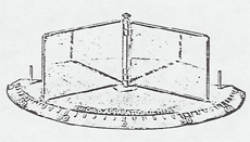
A set of color filters can be projected in a triangular overlapping circle pattern. Filters available are red, blue, green, and minus red, minus blue, and minus green.
The Rav'n light is a small pulsing light that looks white. When swung around on a string you can see that it is made up of only red, green, and blue pulses.
There is a new set of red, green and blue leds which can be projected into overlapping circles. The intensity of each light can be adjusted to some extent to make any color in the overlapping region. An amber led is also available and can be compared to a mixture of red and green. This can be used to discuss how the eyes see color. Why for instance, do red and green light, with no wavelengths in the yellow spectral region, give the sensation of yellow? The answers can be found in the sensitivity of the three types of cones in the eye. Sample led spectra, cone sensitivity, and the CIE diagram are below. The CIE diagram can be used to describe the gamut of any display device. For more info go here. [87]
Also available are hand-held color mixers. One device has a tricolor red, blue and green LED with three switches. By pressing two of the three switches, the secondary or negative colors are made and by pressing all three at the same time we get white light.
Participants at a workshop show the seven possible colors after making this little color mixer with a tricolor led. This is similar to controlling a single pixel of a 3 bit RGB display. Black is the eigth color.
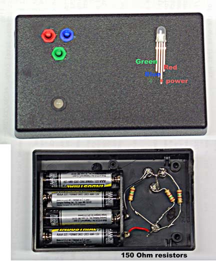
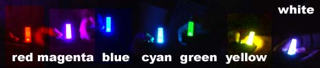
The tri color led can be found here [88].
Color Algebra
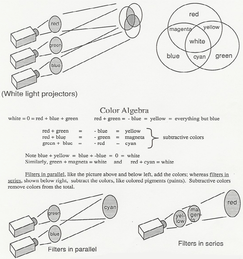
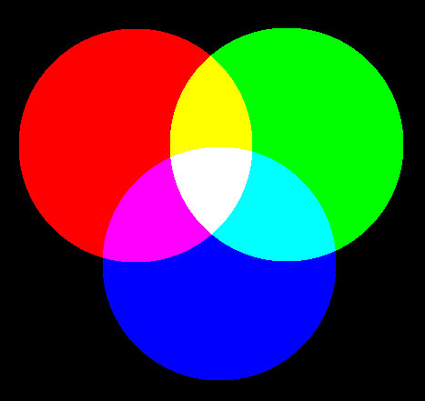
Light from red, green and blue LEDs is projected into overlapping circles. The intensity of each LED light can be adjusted to make white or other colors in the overlapping region.
Spectral colors are characterized by the wavelength of the electromagnetic radiation. The shortest wavelength that can be seen by the eye is 380 nm violet. The longest wavelength which can be seen is 770 nm red. The wavelengths of the light produced by the red, green, and blue LEDs is shown in the top graph, along with that of an amber LED.
One interesting thing to note is that the spectrum of the amber LED does not overlap very much with the spectrum of the red and green LED. The light from the red and green LEDs does not contain any amber wavelengths around 590 nm, yet we see the color amber when we mix red and green light. Why is this?
The answer can be found in the sensitivity of the three types of cones in most peoples eyes (see the second graph). These are sensitive to short, medium, and long wavelengths which roughly correspond to blue, green and red light. Amber light at 590 nm, excites both the green and red cones. We can fool the brain into seeing amber, by supplying the right amount of red and green stimulation. That's why color mixing works. However, everyone's eyes are different. Some people only have two types of cones and have some color blindness. Some reportedly have four types. The ratio of red to green cones varies widely from person to person. The ratio of red and green light to match the spectral 590 nm amber also varies from person to person. We don't all see the same colors.
RGB display devices like TV's and monitors project red, green, and blue light to produce the sensation of all the colors. The CIE diagram shows all the colors that can be perceived by the eye/brain. The spectral colors lie on the white curve identified by wavelength and all the various mixtures appear inside. The color gamut of a display device is that part of the full range of colors that the device can reproduce. The color gamut of the red, green and blue LEDs is the area inside the triangle with vertices at the wavelengths of the LEDs. Colors outside the triangle cannot be matched by mixing the light of those LEDs. How close can we get to spectral amber?
Printer inks, paints, and filters use subtractive rather than additive colors. Instead of red, green, blue, printer primaries are usually cyan, magenta, yellow, and black. Printers also have a color gamut and can't reproduce colors outside their gamut. This can lead to problems when the display gamut doesn't match the printer gamut. Colors that can be seen on the screen can't be printed.
Real: The "UFO shaped Optical Illusion" produces a stunningly real looking 3D image of a small object placed inside it. A laser can be shined right on the image, demonstrating optical reciprocity. The device consists of two parabolic mirrors, each at the focus of the other. The object is placed on the lower mirror at the focus of the upper mirror. Beams from the object diverge to the upper mirror and are reflected parallel down to the lower mirror, whence they are converged up through a hole in the upper mirror to form the image.
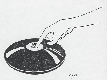
Virtual: In this impressive demonstration the virtual image of the flame of a concealed candle in a sheet of plate glass appears over an unlit candle wick. You can put your finger in the "flame" and grimace, or pour water over it and not put it out
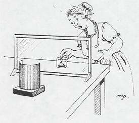
Index of Refraction: With the Blackboard or Whiteboard Optics semicircle piece you can measure the index of refraction of the lucite material directly with Snell's Law This will be a useful value later if you plan to use the rectangular block for parallel deviation or the prism for total internal reflection. Then you can predict and check results from your measured value of n. See Blackboard Optics [89] and Measuring a Glasses Prescription [90].
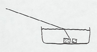
A beam of light is passed through a cell containing precipitated sulfur and then focused on a screen. As the sulfur precipitates, the transmitted beam becomes redder as more and more of the blue light is scattered out of the beam to the sides. The side scattered light can be shown to be polarized.
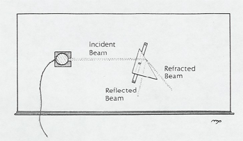
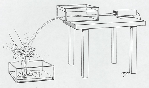
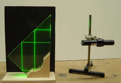
Small ultrasonic piezoelectric transducers serve as transmitters or receivers for centimeter sound waves. A simple setup with two transmitters hooked to the same signal generator produces a very nice interference pattern read out on an oscilloscope. (See Acoustical Interference [43])
A hollow prism filled with carbon disulphide will disperse white light into its component colors. Other glass and lucite prisms are available, but their dispersion is not as great as CS2.
A laser transmission hologram can be set up for individual viewing by the students. One is of a magnifying glass in front of a watch. You can look behind the magnifying glass and see the watch, or look through it and move your eye in and out to see the focus change.
A classic white light "multiplex" image of a woman blowing a kiss is available as well as other reflection type holograms of a microscope, skulls, etc.
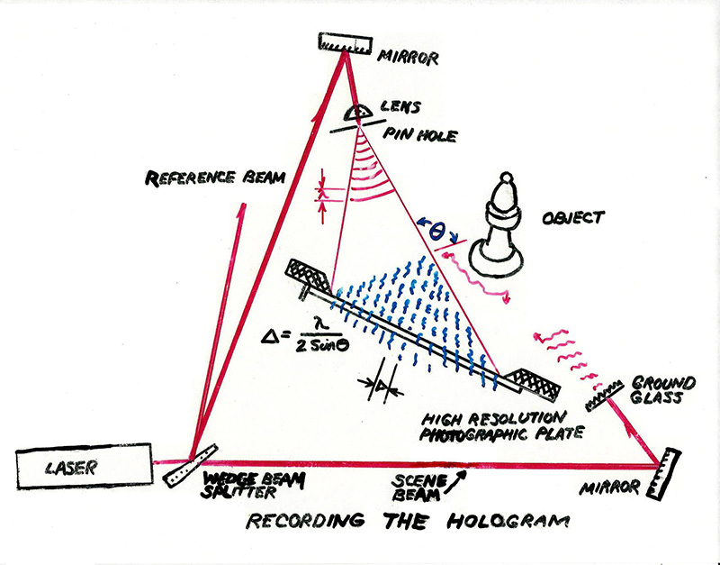
A small interferometer can be demonstrated in class. This is useful when discussing relativity besides the optics application. The fringe pattern can be projected onto the overhead screen, and you can measure the wavelength of the laser light by advancing one of the mirrors with a micrometer screw and counting fringes.
In a very similar setup reflected light from a Newton's rings apparatus is focused on the rear projection screen and the circular colored fringes observed.
Our large ripple tank projects onto the overhead screen to demonstrate reflection, diffraction, interference, etc.
Also available is an PHET applet [92] that nicely demonstrates the interference and diffraction of waves.
A laser beam is arranged to pass through the slits and be reflected onto the overhead screen. Standard demonstrations are single slit diffraction, double slit interference, and diffraction from a circular opening. Two lasers are arranged so that single and multiple slits can be shown simultaneously, one pattern above the other.
We have precision slits etched in metal foil. The slit widths and spacings are marked. The most useful single and double slits have a width of .04 mm. The double slit spacings are .125, .250, and .5 mm. There is also 3, 4, and 5 slits with the same width (0.04 mm) and spacings of .125 mm.
Hair, CD's and DVD's can be used as diffraction gratings. Simple measurements of the first maximum gives the track spacing. Comparing the pattern from CD's and DVD's gives the ratio of the track spacing for the higher density DVD.
The diffration pattern can be observed with both a red and a green laser simultaneously to show the effect of wavelength. The red laser wavelength is 0.6328 micron and the green laser is 0.532 micron.
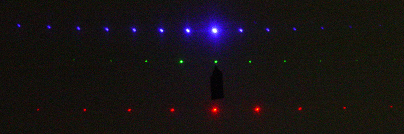
A small ball bearing in a laser beam can show the Arago bright spot (or Poisson spot) in the center of the shadow as seen below. This image also shows the fine structure in the shadow. This demo is best when the students can come right up to the shadow image and look at it directly.
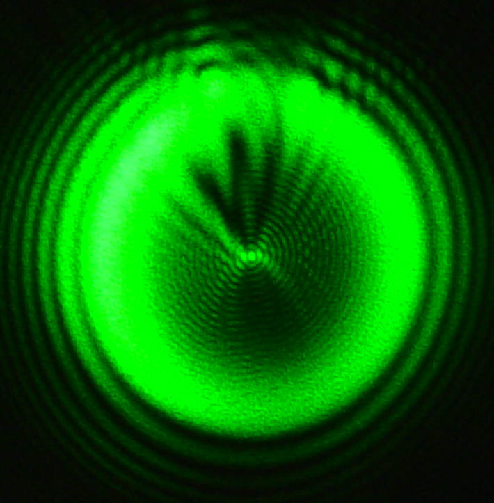
The Cornell plate, diagrammed below can also be used for these demonstrations. It is clipped to a special stand so that successive slits in each column can be brought into the laser beam by adjusting a rack and pinion knob.
Column (a) Successively narrower single slits
Column (e) Successively wider double slits
Column (b) Single slit starts narrow, becomes wider,
becomes double slit, becomes narrower.Column (d) Go from one slit to two slits to three to four to ten to show sharpening
of the fringe maxima.
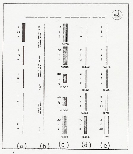
The Cornell plate was originally designed to be used (and can still be used) with the individual eye to view a straight filament bulb.
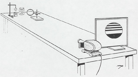
In this pretty demonstration light reflected from a soap film is focused on a rear projection screen. Gravity makes the soap film thicker at the bottom, so the image is a series of colored fringes produced by interference between the light reflected from the front and back surfaces of the film. As the water evaporates, the soap film becomes thinner, and a black area appears at the top of the film (bottom of the screen, if using a lens). When it becomes thinner than 1/4 (lambda/n), it represents destructive interference owing to the 180° phase change at the outside surface. The images below show this effect. (The phase changes at free and fixed ends can be demonstrated with the Bell Wave Machine [93].)

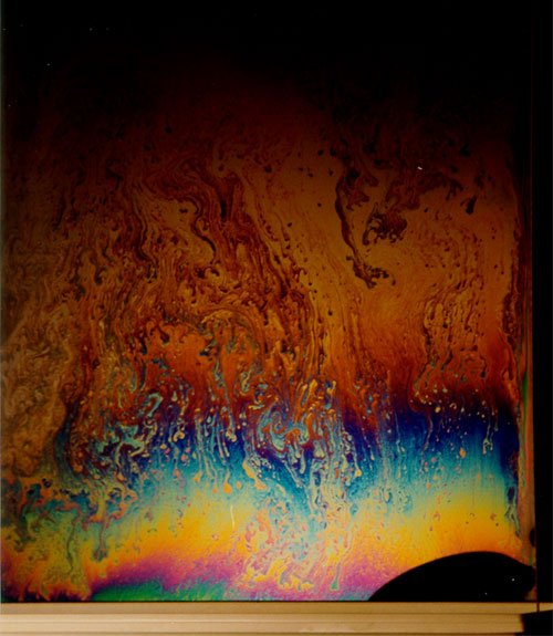
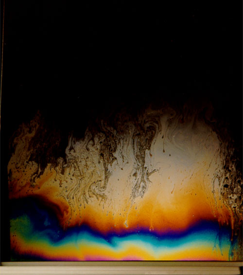
A set of optical instruments is available. Most of them are in a box which you can keep at the front of the class for the students to come down and look at. You have to sort of watch over them to make sure none get dropped or lost. Or you could pass one at a time around and carefully collect it afterwards.
There are opera glasses, which consist of a pair of Galilean telescopes made from a diverging eye lens and a converging objective. This arrangement produces an erect image with only two simple lenses, but at the expense of low power and small field of view. Prism binoculars have converging eye lenses, probably two elements each, with prisms to fold the optical path and erect the image. A pair of Porro prisms is available to show how the inversion of the image is effected, and also a roof prism set is available to show how the same job can be accomplished "in line". A small astronomical telescope produces a bright, clear, wide field image, but upside-down. There is also a "Captain's telescope" with telescoping tubes and an internal converging lens to erect the image. This arrangement produces an erect high power image, but the image is dim and difficult to focus, and the instrument has an unwieldy length.
You can show a microscope and a slide of the lens system of microscopes. Art has a transparency diagram of the elements of the human eye, and there also is a slide of an actual cross-section of an eye. Finally, a demonstration camera with a large plano-convex lens will produce images of lights, etc. in the lecture hall, with some distortion apparent because of the simple lens.
Calcite crystals are available to show the double image of birefringence. One is mounted on a slide projector to produce two circular images from a single hole. As a Polaroid sheet analyzer or the crystal itself is rotated the "extraordinary" and "ordinary" images come in and out of view.
A model of the molecular structure of calcite is also available.
The diagram below shows light entering a birefringent material. Only the E-field is shown, resolved into components along the X- and Y-axis. Upon entering the material light is split into two rays, the ordinary and extraordinary ray, traveling at different velocities. The o-ray and e-ray are plane-polarized along mutually perpendicular directions. The o-ray has polarization perpendicular to the axis of anisotropy and therefore experiences a different index of refraction than the e-ray which has polarization parallel to the axis of anisotropy. The difference in the refraction indices is greatest when the light ray is traveling perpendicular to the axis of anisotropy as portrayed in the diagram. There is an instructive simulation on birefringence available through the website for the PLC project [94] at Case Western Reserve University.
A schematic of a birefringent material showing the axis of anisotropy.
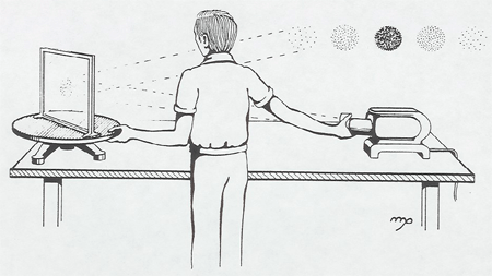
Brewster's angle is nicely demonstrated with the apparatus shown. With the polarizer on the projector horizontal, the reflected beam will be completely extinguished as the glass plate is rotated to Brewster's angle. You can now rotate the polarizer to show polarization of the reflected beam.
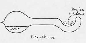
A polarizer and analyzer above and below the bulb end of the cryophorus are crossed to extinguish light transmission and dry ice plus alcohol to increase thermal contact are introduced into the cup end. Rapid evaporation of the water inside the bulb end causes a raft of ice to form. The first time the ice freezes, in about three minutes, many small crystals form at once and jump into view on the overhead screen. The dry ice is now removed, the projector focused carefully, and the cryophorus warmed by hand until the ice melts and the last crystal is just disappearing from the overhead screen. There will still be a few ice crystals left at this point as they melt thinner than the half-wave plate thickness. Dry ice is immediately reintroduced, and in thirty seconds or so beautiful large ice crystals will be seen to grow from the remaining seed crystals, accompanied by Ooh's and Aah's from the class. The demonstration can be repeated several times.
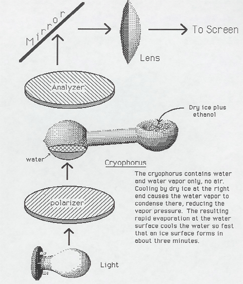
Shown by analyzing light scattered by slide projector. See Sunset Colors from Scattering [95].
Polaroid sheets can be crossed on the overhead projector to show extinction. A third sheet, inserted at 45deg to the other two, will permit 1/8 of the original light to be transmitted. How does inserting a sheet, which can only absorb light, cause more light to be transmitted?
A sodium lamp is arranged to shine on a rear projection screen. An ordinary flame, say of a match or Bunsen burner introduced between the lamp and the screen will not cast a shadow, but if a wire or stick dipped in salt solution is placed in the flame, a dark shadow of the flame appears.
Arc tubes of hydrogen, helium, argon, mercury, and a few others can be viewed three-at-a-time with a large holographic grating. Also available is an incandescent light which can be used to look at a continuous spectrum.

Another option is that students can use individual gratings to see spectral lines of these tubes.
A hollow prism filled with carbon disulphide will disperse white light into its component colors. Other glass and lucite prisms are available, but their dispersion is not as great as CS2.
The action of a diffraction grating itself can be demonstrated by passing a laser beam through the grating and showing the spread out spots on the wall. You can lead into the phenomenon by showing the effect of Single, Double, and Multiple Slits [40] with the Cornell plate. Interesting effects result from crossing two gratings in the laser beam, or by arranging many at all different angles.
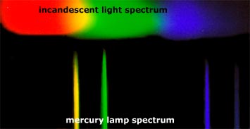
The arrangement below will project the lines of mercury just above their positions in a continuous spectrum of a tungsten filament. By adjusting the height of the 45° mirror you can have the entire length of the mercury lines, mercury lines above continuous spectrum, or just the continuous spectrum. Note that the spectrum of the tungsten filament is deficient in blue as befits a 3000° black body which peaks in the infrared.
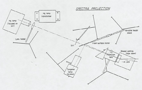
Reference instructions for assistant:
How to measure the speed of light
Winner of 'Great Science Teacher Video Contest' at USA Science and Engineering Festival www.engineering.com

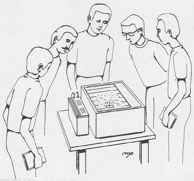
A continuous cloud chamber shows tracks of charged particles. Advance notice is needed to obtain the dry ice necessary to operate the chamber. Thoron gas (thorium emination, Rn 220, half-life = 1 min.) can be blown into the chamber to produce alpha particle tracks. Since the daughter nucleus Po 216 with a half-life of 0.15 sec. is also an alpha-emitter, two pronged tracks will be seen in the chamber. A needle with Pb 210 also produces a-tracks. Two to five students look at this demonstration at once so it is best to arrange a little time at the beginning or end of class for them to come down and look.
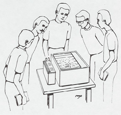
Cloud Chamber
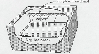
Methanol evaporates from the trough, and the vapor falls toward the cold dry ice (-100 F = -73 C). In the process the vapor is super cooled; that is, cooled below its normal condensation point. When a high speed charged particle from a radioactive source or from a cosmic ray passes through the super cooled vapor, it ionizes the air and methanol atoms along the way; i.e., it strips electrons from these atoms. These ions and electrons serve as condensation centers for the methanol vapor, which condenses out in tiny droplets along the track of the charged particle outlining its path.

The charged particles from the radioactive source are typically helium nuclei (alpha particles). This source is "license free", meaning it is too weak to be considered dangerous by governmental regulatory agencies. Charged particles from cosmic rays are typically protons and muons.
Using the color projector (Projected Colors [97]), you can simulate the quark structure of baryons and mesons.
Heavy water, D2O, molecular weight 20, is about 10% heavier than ordinary water, H2O, molecular weight 18. Identically filled bottles of heavy water and tap water can be compared by hand or on a double pan balance. Of course, deuterium and heavy water are not radioactive.
The Physics Demontrations Group has a collection of videos on nuclear physics including:
The Physics Demontratons Group has a collection of transparencies on nuclear physics copied from Scientific American and other books including:
Small "license free" sources of activity < 0.1 microcurie can be taken into the class to activate a small hand held counter. Cloud chamber alpha sources of lead 210, beta source of strontium 90, thoriated tungsten welding rod, uranium glass (alpha beta gamma), Americium (alpha gamma) from a smoke detector and a hot fiesta ware cup and saucer with uranium glaze are available.
Americium-241, with a half-life of 432 years, is used in most domestic smoke detectors. Am-241 decays by emitting alpha particles and 60 keV gamma radiation to become neptunium-237.
Uranium glass was used to make a yellow tinted dinnerware from Victorian times. Sometimes called Vasoline glass, or depression glass, our bowl measures about 5 µSv/hr. You can tell uranium glass because it fluoresces green under blue or UV light.
Fiesta ware was the largest selling dish line in American history – 200 million dishes were shipped since 1936. The red/orange color glaze contains uranium. The government seized the company's uranium supply in 1943 out of fear it could be used to make a bomb. A single plate contains about 4.5 grams of uranium, mostly U-238. Production resumed in 1959 with depleted uranium (depleted of U-235) and continued until 1972 when it was discontinued out of concerns about uranium and lead leaching out of the glaze. Fiesta ware is the hottest source we have and measures over 100 µSv/hour at the plate surface, but this is not considered dangerous for display purposes. U-238 has a half-life of 4.5 billion years.
Radiation safety standards limit public exposure to 1 mSv/year and occupational exposure to 50 mSv/year. Natural background radiation is about 3 mSv/year.
Contrast that with a typical medical dose as shown below. This reading was taken about two hours after injection with Technetium-99m, a radioisotope used for heart imaging with a 6 hour half life.
A handheld Gieger-Mueller tube is available.
Lewis Carroll Epstein in his book Relativity Visualized has developed several marvelous illustrations curved spacetime. Art has a copy of the book and model transparencies that you can curve and flatten out on the overhead projector to show:
A description of 4-Dimensional space
See Local Inertial Frame (Gravitational Acceleration) [16]. This demonstration is equivalent to the Monkey and Hunter [98] example. A large aluminum frame is cranked up and suspended by a magnet. Two guns on one side of the frame are aimed in straight lines through holes in an intermediate Plexiglas sheet at target pockets on the other side of the frame. If the guns are fired while the frame is suspended, the projectiles travel in parabolas and bounce back from the plastic sheet. But now the guns are reloaded and frame is released to fall. Another switch fires the guns as the cage goes into free fall. When the falling frame is stopped by a "linear decelerator" (a shock absorber) at the bottom, it will be found that the projectiles reached the pockets. In the falling frame, they traveled in straight lines, obeying Newton's First Law.
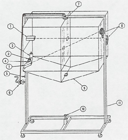
Our device was designed by Dr. R.E. Berg of the University of Maryland (A.J.P. 48, 310 (1980)), and built by the UCLA physics machine shop.
Attention can be called to the well-known Monkey and Hunter [3] demonstration as an illustration of the Principle of Equivalence (POE). The impressive point is that no complicated ballistic calculation is needed. Consider a reference frame falling with the bullet and the monkey. (Imagine a frame released the instant the bullet leaves the muzzle and the monkey starts falling.) In this frame the bullet is initially directed at the monkey and travels uniformly in a straight line toward it. By the POE this falling frame is truly inertial and the fact that the bullet hits the monkey is an immediate consequence of Newton's First Law. (A. Huffman, A.J.P. 48, 314 (1980))
Two very simple demonstrations of weightlessness when falling are described in Weightlessness (Gravitational Acceleration) [99].
This is a 16 minute NASA video of physics experiments in the orbiting laboratory of Sky lab. Weightlessness is well shown, and the rest is a physics 10 level discussion of gravity, satellite motion, and illustrations of Newton's laws in weightlessness.
This demonstration uses the microwave apparatus of experiment 2 in the 8D lab. The microwaves produced by a Gunn diode are picked up by a receiver and indicated on a meter visible to the class. When one of the 45 degree prisms is inserted into the beam, the meter reading drops to near zero - the microwaves have been totally internally reflected at right angles. You can demonstrate that this is the case by moving the receiver around to the right-angle position to pick them up. Now the receiver is returned to the original position, and a second prism is brought close to the first as shown above. When the gap is about one centimeter or less, the signal begins to increase - the microwaves have tunneled across the gap into the second prism. When the gap distance is reduced to zero, the signal reaches its full value. As the gap distance is increased, the signal drops off exponentially.
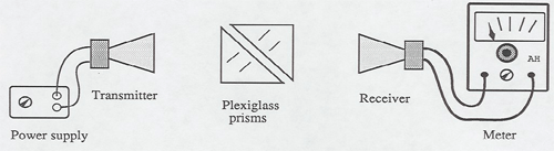
Remember, even electromagnetic microwaves are photons! This is a demonstration of particles penetrating a barrier.
The black body radiation curve can be demonstrated by using a radiation sensor hooked to a digital millivoltmeter. The carbon disulfide prism [73] is used to spread out the light of a slide projector lamp onto a screen . As you scan across the spectrum with the radiation sensor, the millivoltmeter shows the peak of the 3000 K tungsten filament in the infrared with the tails of the curve in the visible spectrum and further infrared.
The same demonstration can be done more qualitatively. Turn down the room lights and show the spectrum of "white" light on the wall. As you reduce the voltage to the lamp with the variac, the blue color dies away, and then the green, leaving only dull red of low intensity. (Of course, the 3000 K tungsten filament already peaks in the infrared so the initial "white" light is already quite red. Infrared itself can be demonstrated; see Infrared, Radiometer, and Maxwell's Spectrum [100])
|
The applet below shows the blackbody curve and colors corresponding to the given temperature. |
|||
|
When introducing the Bohr atom it is a good idea to review standing waves for the students, for example with Rudnick's String [33]. You can show how the string resonates for various harmonics as the driving frequency is changed.
Another demonstration puts standing waves on a circular wire loop - standing waves around a circle. A mechanical wave driver controlled by a function generator shakes the loop at the bottom and it resonates with an odd number of antinodes on the circle at the frequencies:
| Number of antinodes | Frequency (Hz) |
| 3 | 18 |
| 5 | 65 |
| 7 | 140 |
| 9 | 237 |
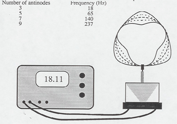
The set-up below is an excellent demonstration of the wave nature of particles. An electron beam is passed through a carbon foil and the resulting diffraction rings displayed on the fluorescent screen of the tube. (Since the graphite crystals are randomly oriented, the diffraction pattern is rings.) From the accelerating voltage, DeBroglie's wavelength, and the diffraction ring diameter, you can calculate the atomic spacing of carbon.
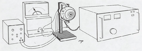
The students don't know what they are seeing. You take that into the class room and the students see green rings, but a physicist sees something astonishing, the wave nature of matter.
-Prof. George Igo
Students can see the spectral lines of hydrogen by looking at a arc tube on the lecture table through replica gratings. Several students can come down at once and look. You can also project the spectrum of mercury on a screen for the whole class to see (See Projected Mercury and Continuous Spectra [101]).
A simple demonstration of energy levels can be done with 4 LEDs, a handcranked generator, and a supercapacitor. As the capacitor is charged by the generator, first the red LED lights, then the green, then the blue. As the capacitor discharges, first the blue led goes dark, then the green, then the red. There is also a fourth IR LED which can't be seen by the eye, but can be seen on a cell phone camera or video camera when the room lights are out. It turns on first and turns off last. Each color has an energy (voltage) threshold which is related to the photon energy. The IR turns on at 1.2 V, red at 1.5 V, green at 2.0 V, and blue at 3.5 V.
The Frank-Hertz Experiment [102] shows atomic energy levels, but it is a very complicated demonstration.
Finally, a very simple demonstration of energy levels is fluorescent and phosphorescent materials with an ultraviolet light. The energetic UV light kicks the electrons up into high levels, and as they jump part way down immediately (fluorescent) or with some seconds of delay (phosphorescent with partially forbidden transitions), the electrons emit visible light of various colors. A green phosphor requires a blue or ultraviolet light to be activated. A red or green LED or laser won't make it glow, but a blue LED will.

This classic 1914 experiment showed the existence of energy levels and their association with spectral lines. It involves an elaborate setup which requires over an hour of warm-up time and calibration. It is best suited for a lab experiment, or you could arrange to have it set up in a lab, and then bring the students in to watch it. Give plenty of extra notice.
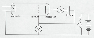
Electrons are accelerated in a nearly evacuated tube with a little mercury vapor in it from the cathode to anode by the voltage V. Those reaching the collector are retarded by 0.5 V. Thus, as V is increased from zero, there is no collector current at A until V > 0.5 V. Then the collector current rises until V reaches the excitation potential of a level in the gas atoms. The inelastic collisions reduce the electrons' energy to zero, and the current drops. As V is increased further, the current again increases until the electrons reach the energy of another level, or double that of the first level. The results can be seen on the current meter as the voltage is increased, or displayed on an oscilloscope screen using a sweep voltage.
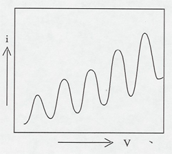
A very simple demonstration of the photoelectric effect is performed with a zinc plate as the electrode of an electroscope. An ultraviolet lamp covered with glass is arranged to shine on the plate. The plate is charged negative with an electrophorus, and the electroscope needle diverges indicating the charge. The blue light of the lamp will not knock out electrons from zinc, but if the glass (opaque to UV) is removed from the lamp, the needle quickly falls as electrons are kicked away from the plate. The zinc plate must be cleaned with steel wool within an hour or so of the demonstration to remove the oxide.
A variation of this experiment has a spiral electrode with a positive voltage in front of the zinc plate with a sensitive current meter to measure the small current of the photoelectrons through the air.
The photoelectric effect is also done as experiment 4 in the 8E lab. The stopping voltage is measured as a function of wavelength (color) of the exciting light, and Planck's constant determined from the slope of the line.
The Ripple Tank [103] is useful to remind the students of wave interference. You might also wish to use the Acoustic Interference [43] demonstration with the ultrasonic transducers. With this setup, you can show that covering one of the two sources will increase the signal to the detector in the case of destructive interference, a key property of waves.
Light has wave properties: show interference with laser shining through slits (See Interference and Diffraction [40]).
Light has particle properties: show the Photoelectric Effect [74].
Electrons have wave properties: show Electron Diffraction [104].
The ratio of e/m for an electron can be measured with an apparatus consisting of a spherical evacuated electron tube mounted inside of a Helmholtz coil setup. The electrons are projected to circle in the magnetic field, and you measure the radius of the circle, the current to the Helmholtz coils, and the accelerating voltage to determine e/m. (See also E/M and Helical Electrons [105].) This is experiment 2 in the 8E lab.
An operating interferometer can be demonstrated in the classroom. It is too small for the actual Michelson-Morley experiment, but you can display to the class interference fringes that change as one of the mirrors is moved.
Two good films for relativity are "Frames of Reference" and "Time Dilation". The first is an excellent older film lasting for 30 minutes showing experiments in Galilean relativity filmed from different points of view, the laboratory frame, uniformly moving, accelerated, and rotating frames. Paul Hewitt's Time Dilation film lasts about 15 minutes and resolves the twin paradox by the Darwin method, counting light signals emitted at regular intervals by the other twin. A description of the twin experiment and calculation of the times is repeated in Hewitt' s book, Conceptual Physics.
Also available are the highly instructive Mechanical Universe series on relativity chapters 42 and 43.
"The influence of the crucial Michelson-Morley experiment on my own efforts has been rather indirect. I learned of it through H.A. Lorentz's decisive investigations of the electrodynamics of moving bodies (1895) with which I was acquainted before developing the special theory of relativity . . . What led me more or less directly to the special theory of relativity was the conviction that the electromotive force acting on a body moving in a magnetic field was nothing else than an electric field.
-Albert Einstein
Although most physicists are aware that relativity is involved in the Faraday magnet and coil induction experiment [75], few exploit the full significance of it as a relativity demonstration. But this experiment demonstrates a truly relativistic effect at very low velocities. It shows, among other things, that physical results depend only on the relative motion (Einstein's first postulate of relativity, the physics is independent of the uniform motion of an inertial frame), and that electric and magnetic fields manifest themselves differently to different moving observers. In addition the experiment has the advantage of motivating relativity in the same way as Einstein was motivated, as in the quote above. This demonstration is useful as a general introduction to relativity in the non-calculus courses and as a motivation for the Lorentz transformation in a higher level special relativity course.
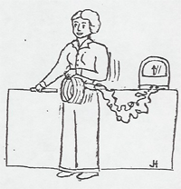
A good place to introduce the demonstration for the first time is just before the coverage of Faraday Induction. (Later when relativity is covered, the demonstration can be repeated and new features emphasized. Referring to the figure first hold the magnet stationary with respect to the classroom, and move the coil toward the magnet. In this situation, case A, the force that moves the electrons around the coil to produce the galvanometer readings the Lorentz force F = qv/c X B. where v is the velocity of the coil toward the magnet.
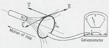
Before demonstrating the moving magnet case B, discuss with the students what they should expect to see. There is a magnetic field, but this does not affect the electrons in the coil, since their velocity is initially zero, and even after they begin to circulate around the coil, the magnetic v X B force is perpendicular to the wire and so does not cause the current. In fact, nothing the students have studied so far in E & M would lead them to expect a galvanometer reading in case B. When this proposition is put to the class, some students will object that " it shouldn't matter whether the coil or magnet is moved". If the class is pressed on this point, one can usually draw out the comment that "only the relative motion should matter". After a short discussion of Einstein's relativity principle, one can go on to perform case B. moving the magnet toward the coil. But, of course, although Einstein's postulate tells us that there must be a new force on the electrons, this new force must have a specific physical origin or description, and it is then appropriate to introduce Faraday induction or Grad X E = 1/c dB/dt. (In a non-calculus course this can be simply worded as a changing magnetic field produces a circular electric field.)
Further points that can be emphasized when the experiment is demonstrated later for relativity are:
The principles of this demonstration as presented in a non-calculus course are summarized on the next page which is available as a transparency from Art.
This demonstration was inspired by section 16.7 of Basic Physics by Kenneth W. Ford (Blaisdell Publishing Co., Waltham, Mass., 1968) The Einstein quote quote at the beginning was from the 1952 meeting honoring the centenary of Michelson's birth as quoted in Introduction to Special Relativity by Robert Resnick (John Wiley and Sons, New York, 1968).
(Art Huffman, AJP 48, 780 (1980))
We see Lucy and Ringo both moving, approaching each other.
Lucy says:
The loop is stationary and the magnet is moving toward it. There is a magnetic field, but it can't produce any force on my electrons since they are stationary within the loop. Instead, the magnetic field is changing, growing stronger as the magnet gets closer, and this changing magnetic field produces an electric field which causes forces on the electrons, and drives them around the loop and produces the current in the galvanometer.
Ringo says:
The magnet is stationary and the loop is moving toward it. The electrons in the loop, since they are moving with the loop, feel a magnetic force, F = - e/c v X B, which drives them around the loop and produces the current in the galvanometer. There is no electric field.
The Conclusion:
Electric and magnetic fields are not invariant entities themselves, but are aspects of a single entity, the electromagnetic field, which manifests itself differently to different moving observers.
This demo consists of a small ball bouncing off a larger ball when both balls are dropped together.
A demonstration of the formation of the solar system or the collapse of a star to a neutron star may be done by using the turntable with weight. A spinning student with weights in her outstretched arms stands on a turntable and brings her arms in. Make sure the student starts off spinning slowly since angular momentum conservation causes the student to spin faster as her arms are brought in.

A gravity well is attached to a rotating platform and spun to simulate binary star systems.
There are two celestial spheres available.
There are various desktop planetarium programs available that can be used with a video projector. These programs can demonstrate the night sky, an orrery of planet motion, retrograde motion, eclipses, etc.
An Earth globe, Moon ball and light bulb for the Sun can be used to demonstrate Moon phases, eclipses, umbra and penumbra.
Two magnetic foci and several different loops are available for drawing ellipses on the blackboard.
- A lead ball at the center deforms an elastic membrane which changes the orbit of a plastic ball. It can be used as a demonstraction of Einstein's general relativity.
- A model of the way gravity distorts space around a heavy object.
The partial pie plate [107]is a good example of what would happen to a satellite if suddenly its host which provides the gravitational force is removed.
Students can see the spectral lines of hydrogen by looking at a arc tube on the lecture table through replica gratings. Several students can come down at once and look. You can also project the spectrum of mercury on a screen for the whole class to see: Projected Mercury and Continuous Spectra [101].
The Frank-Hertz experiment [102] above shows atomic energy levels, but it is a very complicated demonstration.
Finally, a very simple demonstration of energy levels is fluorescent and phosphorescent materials with an ultraviolet light. The energetic UV light kicks the electrons up into high levels, and as they jump part way down immediately (fluorescent) or with some seconds of delay (phosphorescent with partially forbidden transitions), the electrons emit visible light of various colors.
Doppler Shift of sound is dramatically demonstrated by swinging a ringing tuning fork around your head.
The whistle ball is another good way to demonstrate doppler shift. A sponge ball has been stuffed with a battery operated whistle in its core. As the ball is thrown around the lecture hall, the students hear a shift in the ball's frequency.
The action of a diffraction grating itself can be demonstrated by passing a laser beam through the grating and showing the spread out spots on the wall. You can lead into the phenomenon by showing the effect of Single, Double, and Multiple Slits [40] with the Cornell plate. Interesting effects result from crossing two gratings in the laser beam, or by arranging many at all different angles.
A hydrogen arc tube can be viewed with a large holographic grating. Also available is an incandescent light which can be used to look at a continuous spectrum.
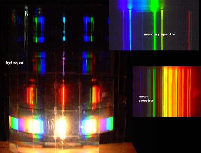
Another option is that students can use individual gratings to see the spectral lines of hydrogen.
A hollow prism filled with carbon disulphide will disperse white light into its component colors. Other glass and lucite prisms are available, but their dispersion is not as great as CS2.
A sodium lamp is arranged to shine on a rear projection screen. An ordinary flame, say of a match or Bunsen burner introduced between the lamp and the screen will not cast a shadow, but if a wire or stick dipped in salt solution is placed in the flame, a dark shadow of the flame appears.
Arc tubes of hydrogen, helium, argon, mercury, and a few others can be viewed three-at-a-time with a large holographic grating. Also available is an incandescent light which can be used to look at a continuous spectrum.
Another option is that students can use individual gratings to see spectral lines of these tubes.
A light bulb with a long filament is powered through a variac on the overhead projector. When the filament is turned down, it looks black against the bright light of the overhead. Then the overhead is turned off and it is shown that the filament is actually glowing and emitting light.
Below are links to suggested demonstrations for Newton's First Law.
A good way to demonstrate Newton's second law is with the Pasco dynamics track [114].
The following demos are recommended to demonstrate the consequences of Newton's Third Law: for every action there is an equal and opposite reaction.
A continuous cloud chamber shows tracks of charged particles. Advance notice is needed to obtain the dry ice necessary to operate the chamber. Thoron gas (thorium emination, Rn 220, half-life = 1 min.) can be blown into the chamber to produce alpha particle tracks. Since the daughter nucleus Po 216 with a half-life of 0.15 sec. is also an alpha-emitter, two pronged tracks will be seen in the chamber. A needle with Pb 210 also produces a-tracks. Two to five students look at this demonstration at once so it is best to arrange a little time at the beginning or end of class for them to come down and look.
Cloud Chamber
Methanol evaporates from the trough, and the vapor falls toward the cold dry ice (-100 F = -73 C). In the process the vapor is super cooled; that is, cooled below its normal condensation point. When a high speed charged particle from a radioactive source or from a cosmic ray passes through the super cooled vapor, it ionizes the air and methanol atoms along the way; i.e., it strips electrons from these atoms. These ions and electrons serve as condensation centers for the methanol vapor, which condenses out in tiny droplets along the track of the charged particle outlining its path.
The charged particles from the radioactive source are typically helium nuclei (alpha particles). This source is "license free", meaning it is too weak to be considered dangerous by governmental regulatory agencies. Charged particles from cosmic rays are typically protons and muons.
Small "license free" sources of activity < 0.1 microcurie can be taken into the class to activate a small hand held counter. Cloud chamber alpha sources of lead 210, beta souse of strontium 90, and an old Coleman gas mantle which contains thorium 232 are available.
A Gieger-Mueller tube simultaneously connected to a counter, an analog meter, and an amplifier and speaker will show the activity of the sources in three different ways.
Experiments 8 and 9 in the 8E lab are concerned with absorption of radiation, half-lives, etc.
Heavy water, D2O, molecular weight 20, is about 10% heavier than ordinary water, H2O, molecular weight 18. Identically filled bottles of heavy water and tap water can be compared by hand or on a double pan balance. Of course, deuterium and heavy water are not radioactive.
The kit has been improved with magnetic clamping to the blackboard and a multiple ray projector. Most of the principles of geometrical optics can be nicely demonstrated with this kit
We have a light which magnetically clamps to the blackboard and projects five parallel rays. This dramatically shows convergence and divergence of rays in lenses and mirrors.
The Lenses and Mirrors applet below can be used as an online demonstration.
Physlet by Wolfgang Christian webPhysics, Davidson College [86]
Instructions on how to use the animation:
A small inverting astronomical telescope can be shown to students individually.
A large parabolic mirror is available to show image formation and to demonstrate how telescopes are used for gathering images.
This demo shows the shifting colors as a function of filament temperature. Also, this demo shows prism dispersion, radiation intensity as a function of wavelength, and infrared radiation. The black body radiation curve can be demonstrated by using a radiation sensor hooked to a digital millivoltmeter. The carbon disulfide prism (see Dispersion [118]) is used to spread out the light of a slide projector lamp onto a screen . As you scan across the spectrum with the radiation sensor, the millivoltmeter shows the peak of the 3000 K tungsten filament in the infrared with the tails of the curve in the visible spectrum and further infrared.
The same demonstration can be done more qualitatively. Turn down the room lights and show the spectrum of "white" light on the wall. As you reduce the voltage to the lamp with the variac, the blue color dies away, and then the green, leaving only dull red of low intensity. (Of course, the 3000 K tungsten filament already peaks in the infrared so the initial "white" light is already quite red. Infrared itself can be demonstrated; see Infrared, Radiometer, and Maxwell's Spectrum [100])
|
The applet below shows the blackbody curve and colors corresponding to the given temperature. |
|||
|
A laser beam is arranged to pass through the slits and be reflected onto the overhead screen. Standard demonstrations are single slit diffraction, double slit interference, and diffraction from a circular opening. Two lasers are arranged so that single and multiple slits can be shown simultaneously, one pattern above the other.
We have precision slits etched in metal foil. The slit widths and spacings are marked. The most useful single and double slits have a width of .04 mm. The double slit spacings are .125, .250, and .5 mm. There is also 3, 4, and 5 slits with the same width (0.04 mm) and spacings of .125 mm.
Hair, CD's and DVD's can be used as diffraction gratings. Simple measurements of the first maximum gives the track spacing. Comparing the pattern from CD's and DVD's gives the ratio of the track spacing for the higher density DVD.
The diffration pattern can be observed with both a red and a green laser simultaneously to show the effect of wavelength. The red laser wavelength is 0.6328 micron and the green laser is 0.532 micron
The Cornell plate, diagrammed below can also be used for these demonstrations. It is clipped to a special stand so that successive slits in each column can be brought into the laser beam by adjusting a rack and pinion knob.
Column (a) Successively narrower single slits
Column (e) Successively wider double slits
Column (b) Single slit starts narrow, becomes wider,
becomes double slit, becomes narrower.Column (d) Go from one slit to two slits to three to four to ten to show sharpening
of the fringe maxima.
The Cornell plate was originally designed to be used (and can still be used) with the individual eye to view a straight filament bulb.
A very simple demonstration of the photoelectric effect is performed with a zinc plate as the electrode of an electroscope. An ultraviolet lamp covered with glass is arranged to shine on the plate. The plate is charged negative with an electrophorus, and the electroscope needle diverges indicating the charge. The blue light of the lamp will not knock out electrons from zinc, but if the glass (opaque to UV) is removed from the lamp, the needle quickly falls as electrons are kicked away from the plate. The zinc plate must be cleaned with steel wool within an hour or so of the demonstration to remove the oxide.
A variation of this experiment has a spiral electrode with a positive voltage in front of the zinc plate with a sensitive current meter to measure the small current of the photoelectrons through the air.
The photoelectric effect is also done as experiment 4 in the 8E lab. The stopping voltage is measured as a function of wavelength (color) of the exciting light, and Planck's constant determined from the slope of the line.
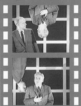
Data Studio is a data acquisition, display and analysis program. The software works with PASCO sensors and interfaces to collect and analyze data in real time. UCLA Physics and Astronomy Lecture Demonstrations has developed numerous experiments for use with undergraduate lectures to demonstrate physics concepts. Some of the concepts that can be shown include the following:
The relation between position, velocity and acceleration (p,v,a plots).
Conservation of momentum and energy.
Heat engines (PV and TS plots).
The relation between pressure and temperature at constant volume (PT at constant V plots).
See our Instructional Videos [119] (also accessible using the tab on the top of the page).
See our ePhysics section at UCLA ePhysics [120].
1. "The Mechanical Universe" is a series of 30 video discs available for the classroom. Also there are VHS tapes for take home viewing.
2. "Encyclopedia of Demonstrations" There are 26 video discs in the series, including one index disc.
3. "Richard Feynman at Cornell University", 1964, a lecture series of 7 different videos is available on DVD and VHS.
4. "Frames of Reference" is available on DVD or you can watch it online here [121].
5. "Powers of 10" by Charles & Ray Eames is available on DVD.
6. "Understanding Car Crashes, it's basic physics" is 22 minutes long and available on VHS.
7. "The Unusual Properties of Liquid Helium", by Isadore Rudnick is 17 minutes long and available VHS.
8. "AAPT Toys in Space", filmed in 1993 on the Space Shuttle, is 60 minutes in length and avaialable on VHS.
9. "Zero G" was filmed at the Sky Lab and available on VHS & DVD.
Check out our YouTube Channel [122].
Links:
[1] https://demoweb.physics.ucla.edu/node/427
[2] https://demoweb.physics.ucla.edu/node/265
[3] https://demoweb.physics.ucla.edu/node/387
[4] https://demoweb.physics.ucla.edu/node/380
[5] https://demoweb.physics.ucla.edu/node/381
[6] https://demoweb.physics.ucla.edu/node/413
[7] https://demoweb.physics.ucla.edu/node/402
[8] https://demoweb.physics.ucla.edu/node/410
[9] https://demoweb.physics.ucla.edu/node/378
[10] https://demoweb.physics.ucla.edu/node/386
[11] https://www.youtube.com/watch?v=92PnUomscGU
[12] https://demoweb.physics.ucla.edu/node/391
[13] https://demoweb.physics.ucla.edu/node/407
[14] https://demoweb.physics.ucla.edu/sites/default/files/demomanual/mechanics/gravitational_acceleration/astronaut.mov
[15] https://demoweb.physics.ucla.edu/node/404
[16] https://demoweb.physics.ucla.edu/node/411
[17] https://demoweb.physics.ucla.edu/node/416
[18] https://demoweb.physics.ucla.edu/node/383
[19] https://demoweb.physics.ucla.edu/node/276
[20] https://demoweb.physics.ucla.edu/node/397
[21] https://demoweb.physics.ucla.edu/node/261
[22] https://demoweb.physics.ucla.edu/node/400
[23] https://demoweb.physics.ucla.edu/node/412
[24] https://demoweb.physics.ucla.edu/node/429
[25] http://ephysics.physics.ucla.edu/newkin/html/position_velocity_ship.htm
[26] https://demoweb.physics.ucla.edu/node/200
[27] https://demoweb.physics.ucla.edu/node/270
[28] https://demoweb.physics.ucla.edu/node/268
[29] https://demoweb.physics.ucla.edu/node/269
[30] https://demoweb.physics.ucla.edu/node/271
[31] https://demoweb.physics.ucla.edu/node/56
[32] https://demoweb.physics.ucla.edu/node/58
[33] https://demoweb.physics.ucla.edu/node/278
[34] https://demoweb.physics.ucla.edu/node/263
[35] https://demoweb.physics.ucla.edu/node/266
[36] https://demoweb.physics.ucla.edu/node/262
[37] https://demoweb.physics.ucla.edu/node/61
[38] http://www.physics.ucla.edu/demoweb/ntnujava/indexPopup.html
[39] https://demoweb.physics.ucla.edu/node/63
[40] https://demoweb.physics.ucla.edu/node/90
[41] https://demoweb.physics.ucla.edu/node/280
[42] https://demoweb.physics.ucla.edu/node/279
[43] https://demoweb.physics.ucla.edu/node/52
[44] https://demoweb.physics.ucla.edu/sites/default/files/demomanual/harmonic_motion_and_waves/waves/spring_wave_long.mov
[45] https://demoweb.physics.ucla.edu/node/53
[46] https://demoweb.physics.ucla.edu/node/55
[47] http://youtube.com/watch?v=ASd0t3n8Bnc
[48] https://demoweb.physics.ucla.edu/chladni_sound.mp4
[49] https://demoweb.physics.ucla.edu/sites/default/files/demomanual/acoustics/effects_of_sound/chladni_sound.mp4
[50] https://demoweb.physics.ucla.edu/sites/default/files/demomanual/acoustics/effects_of_sound/30_MPH_doppler.au
[51] http://ephysics.physics.ucla.edu/physlets/edoppler_shift.htm
[52] https://demoweb.physics.ucla.edu/node/65
[53] https://demoweb.physics.ucla.edu/node/66
[54] https://demoweb.physics.ucla.edu/node/62
[55] https://demoweb.physics.ucla.edu/node/316
[56] http://www.youtube.com/watch?v=-W5FRl0qhOM
[57] https://demoweb.physics.ucla.edu/sites/default/files/demomanual/matter_and_thermodynamics/heat_and_temperature/ln2icecream.jpg
[58] https://demoweb.physics.ucla.edu/node/325
[59] https://demoweb.physics.ucla.edu/node/326
[60] https://demoweb.physics.ucla.edu/node/327
[61] https://demoweb.physics.ucla.edu/node/306
[62] http://ephysics.physics.ucla.edu/brownian-motion
[63] https://demoweb.physics.ucla.edu/node/304
[64] https://demoweb.physics.ucla.edu/node/336
[65] https://demoweb.physics.ucla.edu/node/167
[66] https://demoweb.physics.ucla.edu/node/169
[67] https://demoweb.physics.ucla.edu/node/185
[68] https://demoweb.physics.ucla.edu/node/179
[69] https://demoweb.physics.ucla.edu/node/182
[70] https://demoweb.physics.ucla.edu/node/199
[71] http://www.ntia.doc.gov/osmhome/allochrt.pdf
[72] https://demoweb.physics.ucla.edu/sites/default/files/HertzWavesm.jpg
[73] https://demoweb.physics.ucla.edu/node/208
[74] https://demoweb.physics.ucla.edu/node/209
[75] https://demoweb.physics.ucla.edu/node/197
[76] https://demoweb.physics.ucla.edu/node/205
[77] http://www.richieburnett.co.uk/operation.html
[78] https://demoweb.physics.ucla.edu/node/219
[79] http://www.physics.ucla.edu/marty/levitron/
[80] https://demoweb.physics.ucla.edu/node/165
[81] https://demoweb.physics.ucla.edu/node/249
[82] http://www.ngdc.noaa.gov/seg/geomag/magfield.shtml
[83] https://demoweb.physics.ucla.edu/node/174
[84] https://demoweb.physics.ucla.edu/node/238
[85] https://demoweb.physics.ucla.edu/node/239
[86] http://webphysics.davidson.edu/Applets/Applets.html
[87] https://demoweb.physics.ucla.edu/node/371
[88] http://store.nichia.com/index.asp?PageAction=VIEWPROD&ProdID=52
[89] https://demoweb.physics.ucla.edu/node/362
[90] https://demoweb.physics.ucla.edu/node/367
[91] https://demoweb.physics.ucla.edu/node/360
[92] https://phet.colorado.edu/en/simulation/legacy/wave-interference
[93] https://demoweb.physics.ucla.edu/node/281
[94] http://plc.cwru.edu/tutorial/enhanced/lab/lab.htm
[95] https://demoweb.physics.ucla.edu/node/369
[96] https://demoweb.physics.ucla.edu/sites/default/files/demomanual/optics/SpeedofLight/sol_analysis_i.jpg
[97] https://demoweb.physics.ucla.edu/node/370
[98] https://demoweb.physics.ucla.edu/node/456
[99] https://demoweb.physics.ucla.edu/node/414
[100] https://demoweb.physics.ucla.edu/node/207
[101] https://demoweb.physics.ucla.edu/node/84
[102] https://demoweb.physics.ucla.edu/node/86
[103] https://demoweb.physics.ucla.edu/node/339
[104] https://demoweb.physics.ucla.edu/node/461
[105] https://demoweb.physics.ucla.edu/node/212
[106] http://micro.magnet.fsu.edu/primer/java/scienceopticsu/powersof10/index.html
[107] https://demoweb.physics.ucla.edu/node/79
[108] https://demoweb.physics.ucla.edu/node/150
[109] https://demoweb.physics.ucla.edu/node/100
[110] https://demoweb.physics.ucla.edu/node/151
[111] https://demoweb.physics.ucla.edu/node/102
[112] https://demoweb.physics.ucla.edu/node/101
[113] https://demoweb.physics.ucla.edu/node/99
[114] https://demoweb.physics.ucla.edu/node/104
[115] https://demoweb.physics.ucla.edu/node/146
[116] https://demoweb.physics.ucla.edu/node/148
[117] https://demoweb.physics.ucla.edu/node/149
[118] https://demoweb.physics.ucla.edu/node/293
[119] http://demoweb.physics.ucla.edu/instructional-videos
[120] http://ephysics.physics.ucla.edu/
[121] http://www.archive.org/details/frames_of_reference
[122] http://www.youtube.com/user/uclaphysicsvideo?feature=mhum
[123] https://demoweb.physics.ucla.edu/node/20
[124] https://demoweb.physics.ucla.edu/node/21
[125] https://demoweb.physics.ucla.edu/node/19
[126] https://demoweb.physics.ucla.edu/node/379
[127] https://demoweb.physics.ucla.edu/node/382
[128] https://demoweb.physics.ucla.edu/node/390
[129] https://demoweb.physics.ucla.edu/node/385
[130] https://demoweb.physics.ucla.edu/node/389
[131] https://demoweb.physics.ucla.edu/node/384
[132] https://demoweb.physics.ucla.edu/node/388
[133] https://demoweb.physics.ucla.edu/node/395
[134] https://demoweb.physics.ucla.edu/node/394
[135] https://demoweb.physics.ucla.edu/node/392
[136] https://demoweb.physics.ucla.edu/node/393
[137] https://demoweb.physics.ucla.edu/node/396
[138] https://demoweb.physics.ucla.edu/node/399
[139] https://demoweb.physics.ucla.edu/node/398
[140] https://demoweb.physics.ucla.edu/node/401
[141] https://demoweb.physics.ucla.edu/node/403
[142] https://demoweb.physics.ucla.edu/node/408
[143] https://demoweb.physics.ucla.edu/node/409
[144] https://demoweb.physics.ucla.edu/node/406
[145] https://demoweb.physics.ucla.edu/node/415
[146] https://demoweb.physics.ucla.edu/node/420
[147] https://demoweb.physics.ucla.edu/node/422
[148] https://demoweb.physics.ucla.edu/node/424
[149] https://demoweb.physics.ucla.edu/node/417
[150] https://demoweb.physics.ucla.edu/node/425
[151] https://demoweb.physics.ucla.edu/node/419
[152] https://demoweb.physics.ucla.edu/node/421
[153] https://demoweb.physics.ucla.edu/node/418
[154] https://demoweb.physics.ucla.edu/node/275
[155] https://demoweb.physics.ucla.edu/node/423
[156] https://demoweb.physics.ucla.edu/node/426
[157] https://demoweb.physics.ucla.edu/node/428
[158] https://demoweb.physics.ucla.edu/node/430
[159] https://demoweb.physics.ucla.edu/node/431
[160] https://demoweb.physics.ucla.edu/node/432
[161] https://demoweb.physics.ucla.edu/node/434
[162] https://demoweb.physics.ucla.edu/node/433
[163] https://demoweb.physics.ucla.edu/node/436
[164] https://demoweb.physics.ucla.edu/node/435
[165] https://demoweb.physics.ucla.edu/node/438
[166] https://demoweb.physics.ucla.edu/node/437
[167] https://demoweb.physics.ucla.edu/node/440
[168] https://demoweb.physics.ucla.edu/node/442
[169] https://demoweb.physics.ucla.edu/node/443
[170] https://demoweb.physics.ucla.edu/node/439
[171] https://demoweb.physics.ucla.edu/node/441
[172] https://demoweb.physics.ucla.edu/node/449
[173] https://demoweb.physics.ucla.edu/node/445
[174] https://demoweb.physics.ucla.edu/node/444
[175] https://demoweb.physics.ucla.edu/node/446
[176] https://demoweb.physics.ucla.edu/node/48
[177] https://demoweb.physics.ucla.edu/node/447
[178] https://demoweb.physics.ucla.edu/node/448
[179] https://demoweb.physics.ucla.edu/node/272
[180] https://demoweb.physics.ucla.edu/node/267
[181] https://demoweb.physics.ucla.edu/node/277
[182] https://demoweb.physics.ucla.edu/node/273
[183] https://demoweb.physics.ucla.edu/node/290
[184] https://demoweb.physics.ucla.edu/node/285
[185] https://demoweb.physics.ucla.edu/node/287
[186] https://demoweb.physics.ucla.edu/node/288
[187] https://demoweb.physics.ucla.edu/node/289
[188] https://demoweb.physics.ucla.edu/node/282
[189] https://demoweb.physics.ucla.edu/node/286
[190] https://demoweb.physics.ucla.edu/node/284
[191] https://demoweb.physics.ucla.edu/node/283
[192] https://demoweb.physics.ucla.edu/node/291
[193] https://demoweb.physics.ucla.edu/node/292
[194] https://demoweb.physics.ucla.edu/node/54
[195] https://demoweb.physics.ucla.edu/node/57
[196] https://demoweb.physics.ucla.edu/node/59
[197] https://demoweb.physics.ucla.edu/node/60
[198] https://demoweb.physics.ucla.edu/node/67
[199] https://demoweb.physics.ucla.edu/node/50
[200] https://demoweb.physics.ucla.edu/node/299
[201] https://demoweb.physics.ucla.edu/node/305
[202] https://demoweb.physics.ucla.edu/node/302
[203] https://demoweb.physics.ucla.edu/node/311
[204] https://demoweb.physics.ucla.edu/node/307
[205] https://demoweb.physics.ucla.edu/node/298
[206] https://demoweb.physics.ucla.edu/node/312
[207] https://demoweb.physics.ucla.edu/node/300
[208] https://demoweb.physics.ucla.edu/node/301
[209] https://demoweb.physics.ucla.edu/node/303
[210] https://demoweb.physics.ucla.edu/node/308
[211] https://demoweb.physics.ucla.edu/node/309
[212] https://demoweb.physics.ucla.edu/node/321
[213] https://demoweb.physics.ucla.edu/node/314
[214] https://demoweb.physics.ucla.edu/node/319
[215] https://demoweb.physics.ucla.edu/node/315
[216] https://demoweb.physics.ucla.edu/node/320
[217] https://demoweb.physics.ucla.edu/node/318
[218] https://demoweb.physics.ucla.edu/node/322
[219] https://demoweb.physics.ucla.edu/node/313
[220] https://demoweb.physics.ucla.edu/node/317
[221] https://demoweb.physics.ucla.edu/node/323
[222] https://demoweb.physics.ucla.edu/node/328
[223] https://demoweb.physics.ucla.edu/node/324
[224] https://demoweb.physics.ucla.edu/node/332
[225] https://demoweb.physics.ucla.edu/node/330
[226] https://demoweb.physics.ucla.edu/node/331
[227] https://demoweb.physics.ucla.edu/node/335
[228] https://demoweb.physics.ucla.edu/node/334
[229] https://demoweb.physics.ucla.edu/node/329
[230] https://demoweb.physics.ucla.edu/node/333
[231] https://demoweb.physics.ucla.edu/node/168
[232] https://demoweb.physics.ucla.edu/node/170
[233] https://demoweb.physics.ucla.edu/node/171
[234] https://demoweb.physics.ucla.edu/node/172
[235] https://demoweb.physics.ucla.edu/node/173
[236] https://demoweb.physics.ucla.edu/node/175
[237] https://demoweb.physics.ucla.edu/node/176
[238] https://demoweb.physics.ucla.edu/node/177
[239] https://demoweb.physics.ucla.edu/node/180
[240] https://demoweb.physics.ucla.edu/node/183
[241] https://demoweb.physics.ucla.edu/node/181
[242] https://demoweb.physics.ucla.edu/node/184
[243] https://demoweb.physics.ucla.edu/node/191
[244] https://demoweb.physics.ucla.edu/node/193
[245] https://demoweb.physics.ucla.edu/node/190
[246] https://demoweb.physics.ucla.edu/node/188
[247] https://demoweb.physics.ucla.edu/node/192
[248] https://demoweb.physics.ucla.edu/node/189
[249] https://demoweb.physics.ucla.edu/node/195
[250] https://demoweb.physics.ucla.edu/node/194
[251] https://demoweb.physics.ucla.edu/node/187
[252] https://demoweb.physics.ucla.edu/node/214
[253] https://demoweb.physics.ucla.edu/node/215
[254] https://demoweb.physics.ucla.edu/node/206
[255] https://demoweb.physics.ucla.edu/node/201
[256] https://demoweb.physics.ucla.edu/node/204
[257] https://demoweb.physics.ucla.edu/node/211
[258] https://demoweb.physics.ucla.edu/node/216
[259] https://demoweb.physics.ucla.edu/node/203
[260] https://demoweb.physics.ucla.edu/node/202
[261] https://demoweb.physics.ucla.edu/node/213
[262] https://demoweb.physics.ucla.edu/node/210
[263] https://demoweb.physics.ucla.edu/node/245
[264] https://demoweb.physics.ucla.edu/node/246
[265] https://demoweb.physics.ucla.edu/node/221
[266] https://demoweb.physics.ucla.edu/node/224
[267] https://demoweb.physics.ucla.edu/node/223
[268] https://demoweb.physics.ucla.edu/node/225
[269] https://demoweb.physics.ucla.edu/node/222
[270] https://demoweb.physics.ucla.edu/node/226
[271] https://demoweb.physics.ucla.edu/node/220
[272] https://demoweb.physics.ucla.edu/node/217
[273] https://demoweb.physics.ucla.edu/node/218
[274] https://demoweb.physics.ucla.edu/node/229
[275] https://demoweb.physics.ucla.edu/node/233
[276] https://demoweb.physics.ucla.edu/node/230
[277] https://demoweb.physics.ucla.edu/node/232
[278] https://demoweb.physics.ucla.edu/node/234
[279] https://demoweb.physics.ucla.edu/node/231
[280] https://demoweb.physics.ucla.edu/node/228
[281] https://demoweb.physics.ucla.edu/node/227
[282] https://demoweb.physics.ucla.edu/node/242
[283] https://demoweb.physics.ucla.edu/node/237
[284] https://demoweb.physics.ucla.edu/node/236
[285] https://demoweb.physics.ucla.edu/node/241
[286] https://demoweb.physics.ucla.edu/node/243
[287] https://demoweb.physics.ucla.edu/node/240
[288] https://demoweb.physics.ucla.edu/node/253
[289] https://demoweb.physics.ucla.edu/node/251
[290] https://demoweb.physics.ucla.edu/node/256
[291] https://demoweb.physics.ucla.edu/node/258
[292] https://demoweb.physics.ucla.edu/node/248
[293] https://demoweb.physics.ucla.edu/node/259
[294] https://demoweb.physics.ucla.edu/node/255
[295] https://demoweb.physics.ucla.edu/node/250
[296] https://demoweb.physics.ucla.edu/node/257
[297] https://demoweb.physics.ucla.edu/node/254
[298] https://demoweb.physics.ucla.edu/node/252
[299] https://demoweb.physics.ucla.edu/node/364
[300] https://demoweb.physics.ucla.edu/node/361
[301] https://demoweb.physics.ucla.edu/node/368
[302] https://demoweb.physics.ucla.edu/node/365
[303] https://demoweb.physics.ucla.edu/node/363
[304] https://demoweb.physics.ucla.edu/node/366
[305] https://demoweb.physics.ucla.edu/node/342
[306] https://demoweb.physics.ucla.edu/node/340
[307] https://demoweb.physics.ucla.edu/node/341
[308] https://demoweb.physics.ucla.edu/node/338
[309] https://demoweb.physics.ucla.edu/node/337
[310] https://demoweb.physics.ucla.edu/372
[311] https://demoweb.physics.ucla.edu/node/377
[312] https://demoweb.physics.ucla.edu/node/376
[313] https://demoweb.physics.ucla.edu/node/375
[314] https://demoweb.physics.ucla.edu/node/374
[315] https://demoweb.physics.ucla.edu/node/373
[316] https://demoweb.physics.ucla.edu/node/345
[317] https://demoweb.physics.ucla.edu/node/344
[318] https://demoweb.physics.ucla.edu/node/343
[319] https://demoweb.physics.ucla.edu/node/481
[320] https://demoweb.physics.ucla.edu/node/482
[321] https://demoweb.physics.ucla.edu/node/478
[322] https://demoweb.physics.ucla.edu/node/479
[323] https://demoweb.physics.ucla.edu/node/480
[324] https://demoweb.physics.ucla.edu/node/477
[325] https://demoweb.physics.ucla.edu/node/458
[326] https://demoweb.physics.ucla.edu/node/453
[327] https://demoweb.physics.ucla.edu/node/457
[328] https://demoweb.physics.ucla.edu/node/454
[329] https://demoweb.physics.ucla.edu/node/455
[330] https://demoweb.physics.ucla.edu/node/463
[331] https://demoweb.physics.ucla.edu/node/460
[332] https://demoweb.physics.ucla.edu/node/465
[333] https://demoweb.physics.ucla.edu/node/466
[334] https://demoweb.physics.ucla.edu/node/462
[335] https://demoweb.physics.ucla.edu/node/459
[336] https://demoweb.physics.ucla.edu/node/451
[337] https://demoweb.physics.ucla.edu/node/450
[338] https://demoweb.physics.ucla.edu/node/70
[339] https://demoweb.physics.ucla.edu/node/69
[340] https://demoweb.physics.ucla.edu/book/export/html/2
[341] https://demoweb.physics.ucla.edu/node/74
[342] https://demoweb.physics.ucla.edu/node/75
[343] https://demoweb.physics.ucla.edu/node/73
[344] https://demoweb.physics.ucla.edu/node/78
[345] https://demoweb.physics.ucla.edu/node/77
[346] https://demoweb.physics.ucla.edu/node/80
[347] https://demoweb.physics.ucla.edu/node/87
[348] https://demoweb.physics.ucla.edu/node/88
[349] https://demoweb.physics.ucla.edu/node/91
[350] https://demoweb.physics.ucla.edu/node/92
[351] https://demoweb.physics.ucla.edu/node/93
[352] https://demoweb.physics.ucla.edu/node/94
[353] https://demoweb.physics.ucla.edu/node/95
[354] https://demoweb.physics.ucla.edu/node/96
[355] https://demoweb.physics.ucla.edu/node/98
[356] https://demoweb.physics.ucla.edu/node/105
[357] https://demoweb.physics.ucla.edu/node/144
[358] https://demoweb.physics.ucla.edu/node/153
[359] https://demoweb.physics.ucla.edu/node/154
[360] https://demoweb.physics.ucla.edu/node/155
[361] https://demoweb.physics.ucla.edu/node/157
[362] https://demoweb.physics.ucla.edu/node/158
[363] https://demoweb.physics.ucla.edu/node/159
[364] https://demoweb.physics.ucla.edu/node/161
[365] https://demoweb.physics.ucla.edu/node/162
[366] https://demoweb.physics.ucla.edu/node/163
[367] http://demoweb.physics.ucla.edu/node/502
[368] http://ephysics.physics.ucla.edu
[369] http://www.myphysicslab.com/
[370] http://www.falstad.com/mathphysics.html
[371] http://www.physics.umd.edu/lecdem/
[372] http://www.physics.umd.edu/lecdem/outreach/QOTW/active/questions.htm
[373] http://physicslearning.colorado.edu/PiraHome1.asp
[374] http://www.exploratorium.com/imagery/sounds/30_MPH_doppler.au
[375] http://livephoto.physics.rit.edu/LPVideos/firecracker/firecracker2.mov
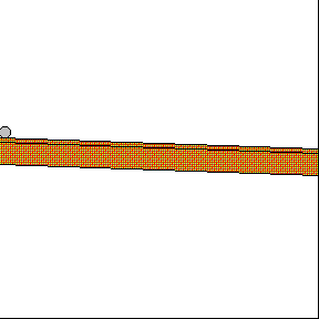
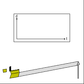
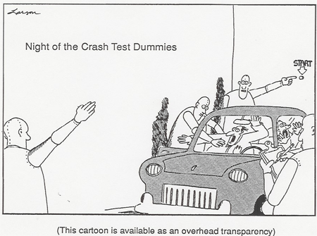


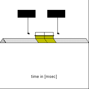
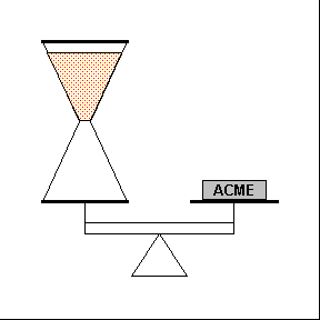
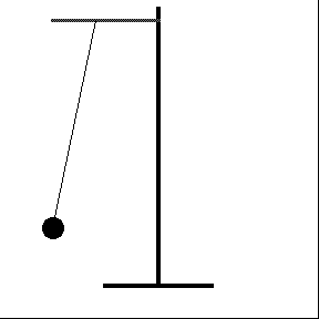
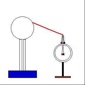
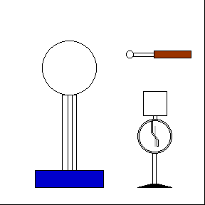
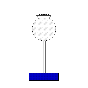
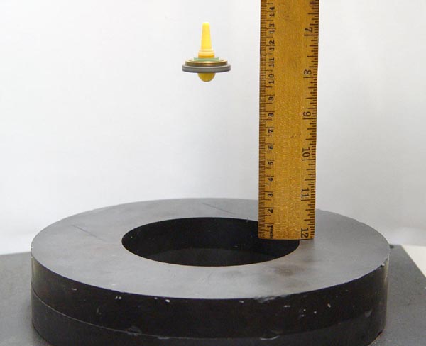
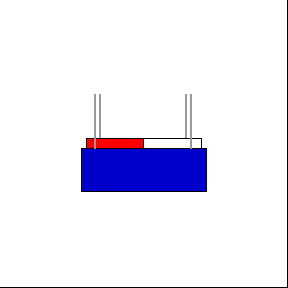
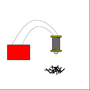
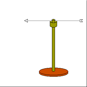